Logistic regression

4. Logistic regression#

Regression is cool and all, but let’s face it: classification is the real deal. I won’t speculate on the distribution of actual problems, but it’s safe to say that classification problems take a massive bite out of the cake.

In this chapter, we’ll learn and implement our very first classification tool. Consider the problem of predicting whether or not a student will pass an exam given the time spent studying; that is, our independent variable $ x \in \mathbb{R} $ quantifies the number of hours studied, while the dependent variable $ y \in \{0, 1\} $ marks if the student has failed ($ 0 $) or passed ($ 1 $) the exam.

We’ll read the data from a .csv using pandas. Don’t worry about the technical details of reading a .csv file; it’s not what we’re here for.

import numpy as np
import pandas as pd
import matplotlib.pyplot as plt

df = pd.read_csv("./logistic-regression-data.csv")
X_train = df["hours"].to_numpy()
Y_train = df["pass"].to_numpy()

Y_train

array([0, 0, 1, 0, 1, 0, 1, 0, 0, 0, 0, 0, 0, 1, 0, 0, 0, 0, 0, 0, 0, 0,
       0, 0, 0, 0, 0, 0, 1, 1, 1, 1, 1, 1, 1, 1, 1, 1, 1, 1, 0, 1, 1, 1,
       1, 1])

No matter the problem, the first step is always visual exploration. (Even when it seems impossible. Get creative and find a way.)

We have an easy job here: make a scatterplot from the $ (x_i, y_i) $-s.

../_images/577f9b84bf1b309906f27d39d25cbeb330046446af8bb28fe15de4c925519e86.png

How can we whip up a classifier that takes a float and conjures a prediction about the success of the exam?

Mathematically speaking, we are looking for a function $ h(x): \mathbb{R} \to \{0, 1\} $, where $ h(x) = 0 $ means that a student who studied $ x $ hours is predicted to fail, while $ h(x) = 1 $ predicts a pass. Again, two key design choices determine our machine learning model:

the family of functions we pick our $ h $ from (that is, our hypothesis space),
and the measure of fit. (That is, our loss function.)

There are several avenues to take. For one, we could look for a function $ h(x; c) $ of a single variable $ x $ and a real parameter $ c $, defined by

\[\begin{split} h(x; c) = \begin{cases} 0 & \text{if } x < c, \\ 1 & \text{otherwise}, \end{cases} \end{split}\]

then find the $ c $ that maximizes the true positive rate

\[ TPR = \frac{\#\text{true positives}}{\#\text{true positives} + \#\text{false negatives}}. \]

This avenue would lead us to decision trees, a simple, beautiful, and extremely powerful family of algorithms routinely beating Starfleet-class deep learning models on tabular datasets. We’ll travel this road later on our journey. For now, we’ll take another junction, the one towards logistic regression. Yes, you read correctly. Logistic regression. Despite its name, it’s actually a binary classification algorithm.

Let’s see what it is!

4.1. The logistic regression model#

One of the most useful principles of problem solving: generalizing the problem sometimes yields a simpler solution.

We can apply this principle by noticing that the labels 0 (fail) and 1 (pass) can be viewed as probabilities. Instead of predicting a mere class label, let’s estimate the probability of passing the exam! In other words, we are looking for a function $ h(x): \mathbb{R} \to [0, 1] $, whose output we interpret as

\[\begin{split} \mathrm{prediction} = \begin{cases} 0, & \text{if } h(x) \leq \frac{1}{2}, \\ 1, & \text{if } h(x) > \frac{1}{2}. \end{cases} \end{split}\]

(In yet another words, we are performing a regression on probabilities.)

Remark 4.1 (The decision cut-off.)

Sometimes, we want to be stricter or looser with our decisions. In general, our prediction can be $$ \mathrm{prediction} = \begin{cases} 0, & \text{if } h(x) \leq c, \\ 1, & \text{if } h(x) > c \end{cases} $$

for the cut-off $ c \in [0, 1] $. Intuitively speaking, the higher $ c $ is, the more evidence we require for a positive classification. For instance, when building a skin cancer detector, we want to be as certain as possible before giving a positive diagnosis. (See the Decision Theory chapter of [Bis06] for more on this topic.)

The simplest way to turn a real number - like the number of study hours - is to apply the sigmoid function

\[ \sigma(x) := \frac{1}{1 + e^{-x}}. \]

Here is its NumPy implementation.

def sigmoid(x):
  return 1/(1 + np.exp(-x))

Let’s see what we are talking about.

../_images/4bbf314db7e8b9d8369b9da10684bf786bcddc6fb4b488c933f9111842978986.png

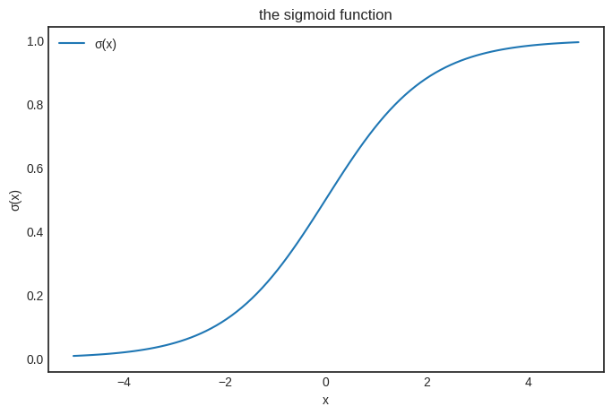
The behavior of sigmoid is straight-forward:

\[\begin{split} \sigma(x) \begin{cases} < \frac{1}{2} & \text{if } x < 0, \\ = \frac{1}{2} & \text{if } x = 0, \\ > \frac{1}{2} & \text{if } x > 0. \end{cases} \end{split}\]

From the perspective of binary classification, this can be translated to

predicting $ 0 $ if $ x \leq 0 $,
and predicting $ 1 $ if $ x > 0 $.

In yet another words, $ 0 $ is the decision boundary of the simple model $ \sigma(x) $. Can we parametrize the sigmoid to learn the decision boundary for our fail-or-pass binary classification problem?

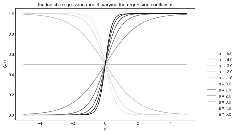
A natural idea is to look for a function $ h(x) = \sigma(ax + b) $. You can think about this as

turning the study hours feature $ x $ into a score $ ax + b $ that quantifies the effect of $ x $ on the result of the exam,
then turning the score $ ax + b $ into a probability $ \sigma(ax + b) $.

(The model $ h(x) = \sigma(ax + b) $ is called logistic regression because the term “logistic function” is an alias for the sigmoid, and we are performing a regression on probabilities.)

Let’s analyze $ h(x) $.

def h(x, a, b):
    return sigmoid(a*x + b)

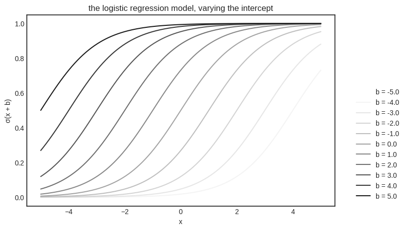
Geometrically speaking, the regression coefficient $ a $ is responsible for how fast the probability shifts from $ 0 $ to $ 1 $, while the intercept $ b $ controls where it happens. To illustrate, let’s vary $ a $ and fix $ b $.

../_images/26447132dc44bbe3a9e212e85c7a23f38733d4e75e441e6ed01c65ba216393c2.png

Similarly, we can fix $ a $ and vary $ b $.

../_images/ca2fef8da622891677370be6d7b8286af119e272784f39bb5d1f5835ca30157e.png

So, we finally have a hypothesis space

\[ \mathcal{H} = \{ \sigma(ax + b): a, b \in \mathbb{R} \}. \]

How can we find the single function that fits our data best?

4.1.1. The binary cross-entropy loss#

Now that we have a model, we need a measure of fit. For linear regression, we have used the mean squared error, defined by

\[ \mathrm{MSE}(h, \mathcal{D}) = \frac{1}{n} \sum_{i=1}^{n} \big( h(x_i; a, b) - y_i \big)^2, \]

where $ x_i \in \mathbb{R} $ is the number of study hours, $ y_i \in {0, 1} $ is the grade of the $ i $-th student, and

\[ \mathcal{D} = \{ (x_i, y_i): i = 1, \dots, n \} \]

is the training dataset. Syntactically, the mean squared error works, but it is not designed to handle probabilities. Think of the loss function as a distance on a space of functions. When the hypothesis functions output probabilities, the mean squared error is distorted.

In the case of (binary) classification, we want to compare probability distributions. (As opposed to point estimates, like we did for regression.) To be more precise, we have the Bernoulli distributions $ (1 - y_i, y_i) $ for the ground truth $ y_i $ and $ (1 - h(x_i), h(x_i)) $ for the prediction $ h(x_i) $.

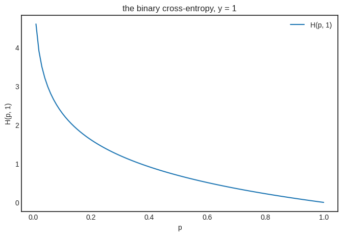
This can be done with the binary cross-entropy, defined by

\[ H(h, x_i, y_i) = - \Big[ y_i \log h(x_i) + (1 - y_i) \log (1 - h(x_i)) \Big]. \]

Let’s unpack this formula. We’ll start with an intuitive explanation before hitting the theory. (Spoiler alert: it is derived from the maximum likelihood estimation.)

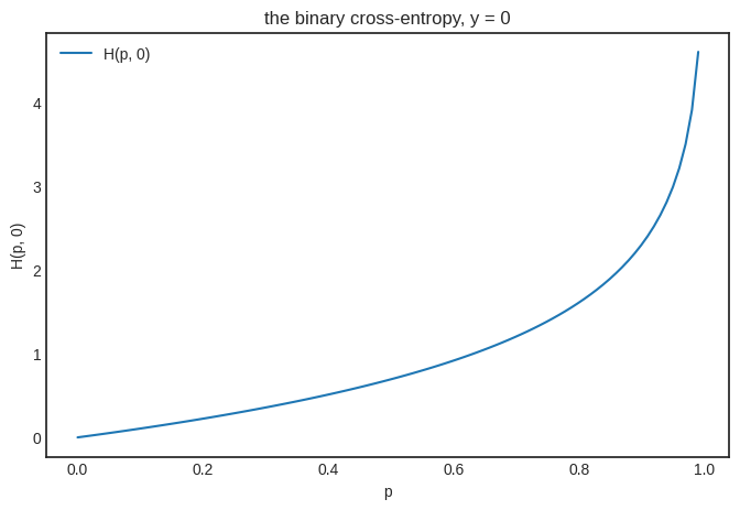
First, note that the binary cross-entropy can be written as the function of $ p = h(x) $, taking the form

\[ H(p, y) = - \Big[ y \log p + (1 - y) \log (1 - p) \Big]. \]

In our case, $ y $ can be either zero or one. If $ y = 1 $, we simply have $ H(p, 1) = - \log p $. This is a decreasing function, assigning a larger loss to smaller $ p $. (Making perfect sense, as $ y = 1 $ is the ground truth.)

../_images/a388c44f97702cde9e9bacfc47a3fa1f407952193186d43d29b5595d1ad54b86.png

As you would expect, things change for $ y = 0 $, yielding an increasing function that punishes the prediction $ p $ as it goes further from the ground truth $ y = 0 $.

../_images/768c5c0401589f27e4ca61c41b53895aba493aaa3ad3c3026afb4100a5e43a0d.png

Now that we have a way to measure the loss of each prediction, we can average them together to obtain the binary cross-entropy loss defined by

\[\begin{split} \begin{align*} \mathrm{BCE}(h, \mathcal{D}) &= \frac{1}{n} \sum_{i=1}^{n} H(h, x_i, y_i) \\ &= - \frac{1}{n} \sum_{i=1}^{n} \Big[ y_i \log h(x_i) + (1 - y_i) \log (1 - h(x_i)) \Big], \end{align*} \end{split}\]

where $ \mathcal{D} = \{ (x_i, y_i): i = 1, \dots, n \} $ is our training dataset.

4.2. Fitting the model#

To find the best fit, we employ the same strategy that we did for linear regression: minimizing the loss function

(4.1)#\[\begin{split} \begin{align*} L(a, b) &= \mathrm{BCE}(h, \mathcal{D}) \\ &= - \frac{1}{n} \sum_{i=1}^{n} \Big[ y_i \log \sigma(a x_i + b) + (1 - y_i) \log (1 - \sigma(a x_i + b)) \Big] \end{align*} \end{split}\]

via gradient descent. To compute the gradient, let’s start with a building block that’ll certainly appear in $ \nabla L(a, b) $: the sigmoid’s derivative. With the single-variable chain rule, we have

(4.2)#\[\begin{split} \begin{align*} \frac{d}{dx} \sigma(x) &= \frac{d}{dx} \frac{1}{1 + e^{-x}} \\ &= \frac{e^{-x}}{(1 + e^{-x})^2} \\ &= \sigma(x) (1 - \sigma(x)). \end{align*} \end{split}\]

Thus, we have

\[ \begin{align*} \frac{\partial L}{\partial a} = - \sum_{i=1}^{n} \Big[ y_i \frac{\partial}{\partial a} \log \sigma(a x_i + b) + (1 - y_i) \frac{\partial}{\partial a} \log \big(1 - \sigma(a x_i + b)\big) \Big]. \end{align*} \]

(Where we used the fact that differentiation is interchangeable with addition and constant multiplication.) Using the chain rule and the fact that $ \sigma^\prime(x) = \sigma(x) \big(1 - \sigma(x)\big) $, we get

\[\begin{split} \begin{align*} \frac{\partial}{\partial a} \log \sigma(a x_i + b) &= \frac{1}{\sigma(a x_i + b)} \frac{\partial}{\partial a} \sigma(a x_i + b) \\ &= x_i \frac{\sigma^\prime(a x_i + b)}{\sigma(a x_i + b)} \\ &= x_i \frac{ \sigma(a x_i + b) \big(1 - \sigma(a x_i + b) \big)}{\sigma(a x_i + b)} \\ &= x_i \big( 1 - \sigma(a x_i + b)\big), \end{align*} \end{split}\]

and similarly,

\[ \frac{\partial}{\partial a} \log \big(1 -\sigma(a x_i + b)\big) = x_i \sigma(a x_i + b). \]

Combining these (and a similar argument for $ \frac{\partial L}{\partial b} $), we get

\[\begin{split} \begin{align*} \frac{\partial L}{\partial a} &= \sum_{i=1}^{n} x_i \Big[ \sigma(a x_i + b) - y_i \Big], \\ \frac{\partial L}{\partial b} &= \sum_{i=1}^{n} \Big[ \sigma(a x_i + b) - y_i \Big]. \end{align*} \end{split}\]

To have everything in one place, here are our implementations of $ h(x, a, b) $, $ L(a, b) $, and $ \nabla L(a, b) $.

def h(x, a, b):
    return sigmoid(a*x + b)

def L(a, b, X, Y):
    n = len(X)
    return -sum([y*np.log(h(x, a, b)) + (1 - y)*np.log(1 - h(x, a, b)) 
                 for x, y in zip(X, Y)])/n

def grad_L(a, b, X, Y):
    n = len(X)
    da = sum([x*(h(x, a, b) - y) for x, y in zip(X, Y)])
    db = sum([h(x, a, b) - y for x, y in zip(X, Y)])
    return (da, db)

Once more, we’ll run gradient descent: with the notation $ \mathbf{w} = (a, b) $, we

select a set of initial parameters $ \mathbf{w}_0 $,
then iterate $ \mathbf{w}_{k+1} = \mathbf{w}_k - \alpha \nabla L(\mathbf{w}_k) $ until convergence,

with learning rate $ \alpha > 0 $.

a_0, b_0 = (0.0, 0.0)    # the initial parameters
lr = 0.01                # the learning rate
n_steps = 2000           # the number of optimization steps
ws = [(a_0, b_0)]        # we'll keep our parameters in the list ws

for _ in range(n_steps):
    a_k, b_k = ws[-1]
    da, db = grad_L(a_k, b_k, X_train, Y_train)
    ws.append((a_k - lr*da, b_k - lr*db))

(These four cells above contain only 18 lines of code, yet they implement a fully functional logistic regression algorithm. We are able to write such clear and efficient code by understanding the algorithms down to their core.)

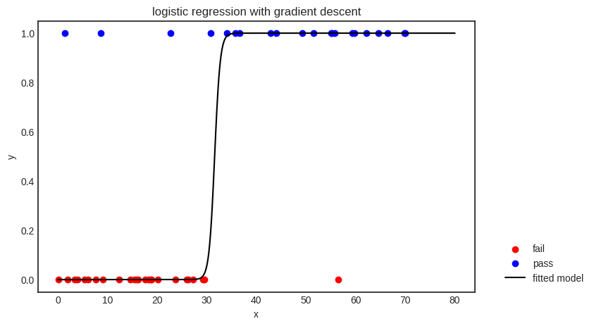
Checking the result.

f"h(x) = {ws[-1][0]} x + {ws[-1][1]}"

'h(x) = 1.7870560236989759 x + -56.46937224709322'

../_images/6063e38cefdf1901b0e519c290646eeebed32bf0c0b1edd78cce7aabe6dbc8a9.png

The decision boundary is given by $ x = -b/a $ (via solving $ ax + b = 0 $), splitting the feature space into two parts: $ x \leq -b/a $, where the points are classified as “fail”, and $ x > -b/a $, where the model predicts “pass”.

../_images/58752850e34f427423ac4e93e9213a8b248e2d23c152590f618906b9c5e60e4e.png

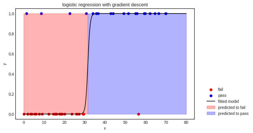
As you can see, the model is not perfect; it even misclassifies a few training samples. There are a couple of potential reasons for this; for instance, 1) the model is not complex enough to represent the relationship between the variables, or 2) the features are not enough to extract any meaningful relationship between the input and the output.

This book is dedicated to solving this problem by building more descriptive models. Don’t be mistaken, though: data engineering is absolutely essential. (Grammarly suggested that the word “absolutely” is redundant in “absolutely essential”. I refused to remove it. Data engineering is absolutely essential.)

4.3. Logistic regression as a maximum likelihood estimation#

We’ve left off the last chapter by showing that linear regression is a statistical model in disguise: fitting a linear function using the mean squared error is the same as fitting a Gaussian process (with linear expectation) via the maximum likelihood estimation.

As we are about to see, logistic regression with the binary cross-entropy loss also originates from our good old friend, the maximum likelihood estimation. This time, our statistical model assumes that the target variable follows a Bernoulli distribution. That is, just like for linear regression, if the inputs $ x_1, \dots, x_n $ are coming from the distribution of $ X $ and the outputs $ y_1, \dots, y_n $ are coming from $ Y $, then the conditional distribution of $ Y $ given $ X $ is described by

\[ P(Y = y \mid X = x) = p(x)^{y} (1 - p(x))^{1 - y}, \]

where $ p = p(x) $ is the parameter of our conditional distribution for the input $ x $.

So, the likelihood function is given by

\[\begin{split} \begin{align*} \mathrm{LLH}(p) &= \prod_{i=1}^{n} P(Y = y_i \mid X = x_i) \\ &= \prod_{i=1}^{n} p(x_i)^{y_i} (1 - p(x_i))^{1 - y_i}. \end{align*} \end{split}\]

Again, we are using the same old trick: taking the log to turn the product into a sum. Thus, we obtain

\[\begin{split} \begin{align*} \log \mathrm{LLH}(p) &= \log \bigg[ \prod_{i=1}^{n} p(x_i)^{y_i} (1 - p(x_i))^{1 - y_i} \bigg] \\ &= \sum_{i=1}^{n} \log \bigg[ p(x_i)^{y_i} (1 - p(x_i))^{1 - y_i} \bigg] \\ &= \sum_{i=1}^{n} \Big[ y_i \log p(x_i) + (1 - y_i) \log (1 - p(x_i)) \Big]. \end{align*} \end{split}\]

We are almost there; the fingerprint of binary cross-entropy is already apparent. If our hypothesis takes the logistic form $ p(x) = \sigma(ax + b) $, the log-likelihood $ \log \mathrm{LLH}(p) = \log \mathrm{LLH}(a, b) $ can be written as

\[ \log \mathrm{LLH}(a, b) = \sum_{i=1}^{n} \Big[ y_i \log \sigma(a x_i + b) + (1 - y_i) \log (1 - \sigma(a x_i + b)) \Big]. \]

This is the same story we have seen dozens of times. (So much so that I am running out of phrases to indicate this.) Maximizing the log-likelihood is the same as minimizing its negative, and adding a multiplicative scaling factor doesn’t change the location of the extrema either. Thus, the minima of

\[\begin{split} \begin{align*} L(a, b) &= - \frac{1}{n} \log \mathrm{LLH}(a, b) \\ &= - \frac{1}{n} \sum_{i=1}^{n} \Big[ y_i \log \sigma(a x_i + b) + (1 - y_i) \log (1 - \sigma(a x_i + b)) \Big] \end{align*} \end{split}\]

gives both the optimal parameters for the logistic regression model $ \sigma(ax + b) $ and the maximum likelihood estimate for our Bernoulli distributions.