7. Computational graphs#
In computer science and mathematics, constructing a new representation of an old concept can kickstart new fields. One of my favorite examples is the connection between graphs and matrices: representing one as the other has proven to be extremely fruitful for both objects. Translating graph theory to linear algebra and vice versa was the key to numerous hard problems.
What does this have to do with machine learning? If you have ever seen a neural network, you know the answer.
From a purely mathematical standpoint, a neural network is a composition of a sequence of functions, say,
whatever those mystical \( \mathrm{Softmax}\), \(\mathrm{Linear}\), and \( \mathrm{ReLU} \) functions might be.
On the other hand, take a look at this figure below. Chances are, you have already seen something like this.
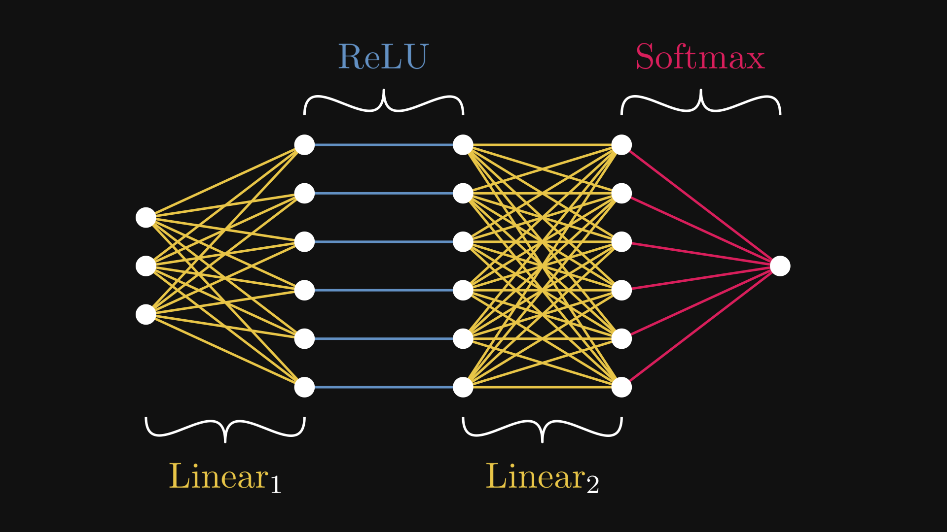
Fig. 7.1 The example neural network \( N = \mathrm{Softmax} \circ \mathrm{Linear}_2 \circ \mathrm{ReLU} \circ \mathrm{Linear}_1 \)#
Fig. 7.1 is the computational graph representation of the neural network \( N \). While the expression (7.1) describes \( N \) on the macro level, Fig. 7.1 zooms into the micro domain.
This is more than just a fun visualization tool. Computational graphs provide us with a way to manage the complexity of large models like a deep neural network.
To give you a taste of how badly we need this, try calculating the derivative of \( N(\mathbf{x}) \) by hand. Doing this on paper is daunting enough, let alone provide an efficient implementation. Computational graphs solve this problem brilliantly, and in the process, they make machine learning computationally feasible.
Here are the what, why, and how of computational graphs.
7.1. What is a computational graph?#
Let’s go back to square one and take a look at the expression \( c(a + b) \). Although this merely seems like a three-variable function defined by
we can decompose it further, down to its computational atoms. Unraveling the formula, we see that \( f \) is the composition of the two functions \( f_1(a, b) = a + b \) and \( f_2(a, b) = a b \) via
Even though this is a simple example, the expression \( f_2\big(c, f_1(a, b)\big) \) is already not the nicest to look at. You can imagine how quickly the complexity slips out of control; just try to re-write \( (a + b)\big(e(c + d) + f\big) \) in the same manner. So, we need a more expressive notation.
What if, instead of using an algebraic expression, we build a graph where the components \( a \), \( b \), \( c \), \( f_1 \), and \( f_2 \) are nodes, and the connections represent the inputs to each component?
It’s easier to show than tell, so this is what I am talking about.
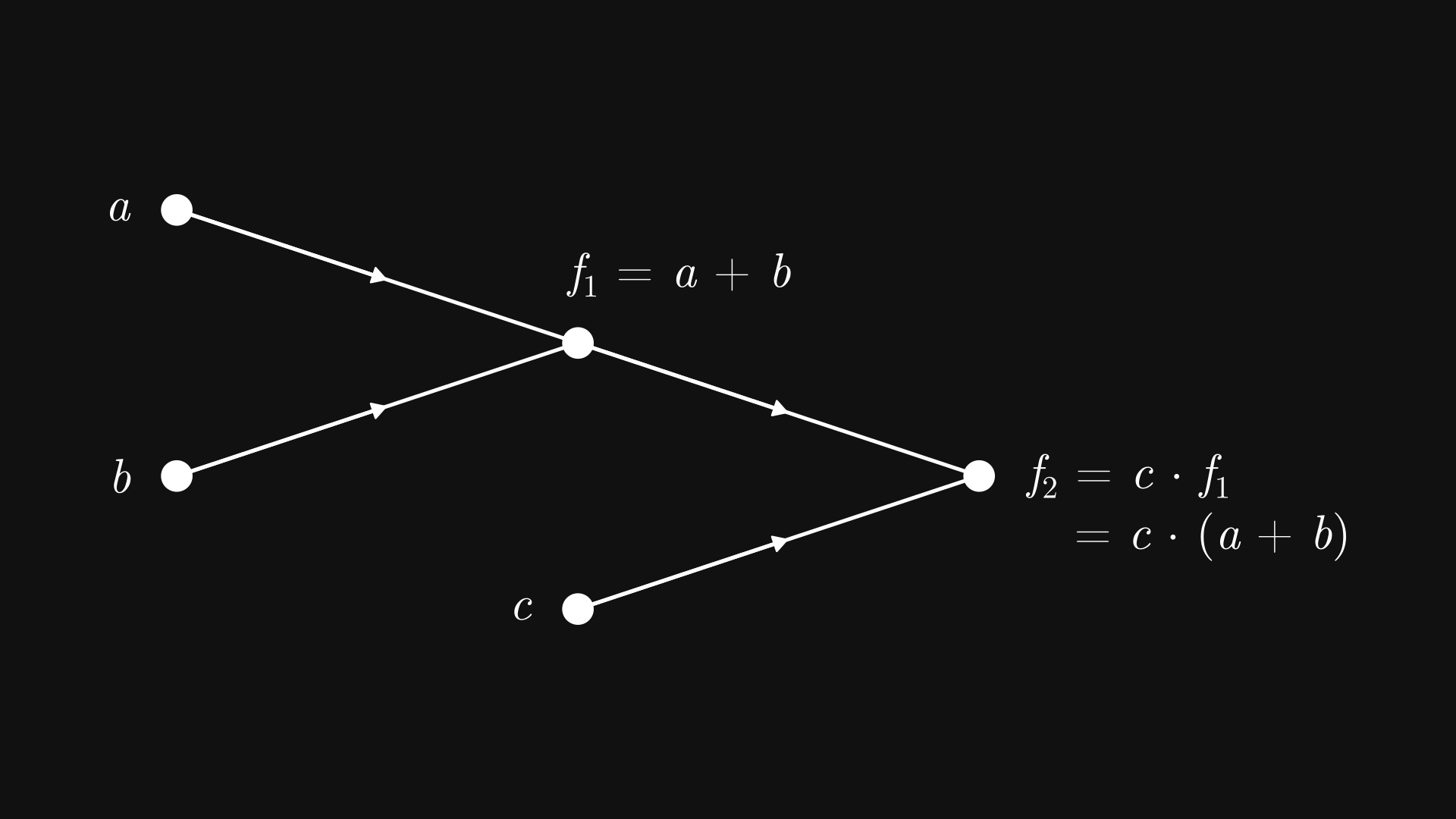
Fig. 7.2 The computational graph of \( c (a + b) \)#
In other words, Fig. 7.2 depicts a tree graph, where
the leaf nodes (such as \( a \), \( b \), and \( c \)) are the input variables,
and the inner nodes (such as \( f_1 \) and \( f_2 \)) are computations, with the children nodes as the inputs.
Because this bears a resemblance to how brain cells communicate, these nodes are called neurons. Hence the term neural network, which is just a fancy name for computational graphs.
Now, the graph Fig. 7.2 is just a symbolic representation for the function \( f(a, b, c) = c(a + b) \). How do we perform the actual computations? We start from the inputs at the leaf nodes, and work our way up step by step. Here’s an illustration using our recurring example \( c (a + b) \) with the inputs \( a = 1 \), \( b = 3 \), and \( c = 2 \). Upon initialization, the computation takes two steps to complete.
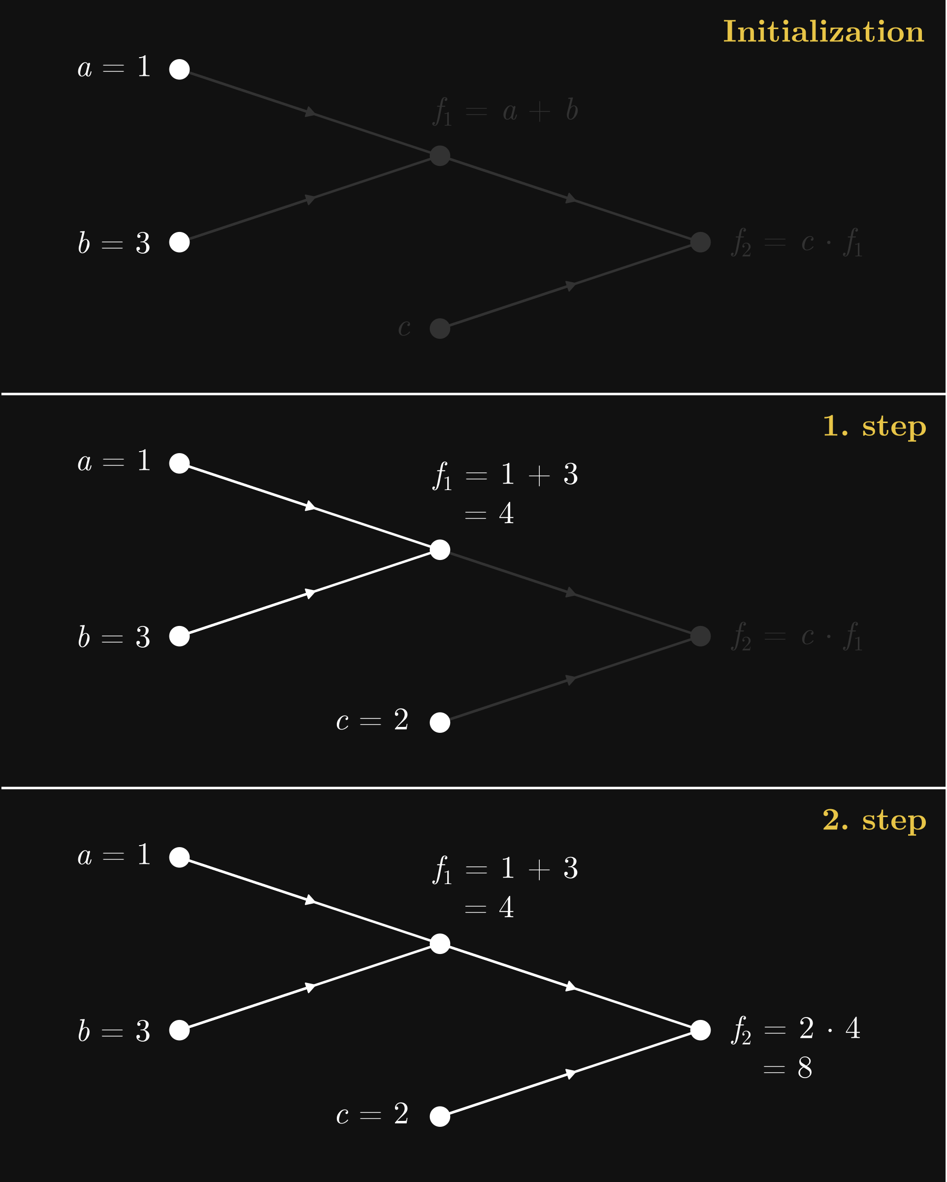
Fig. 7.3 The forward pass in the computational graph of \( c (a + b) \)#
This process is called the forward pass, as with each step, we propagate the initial values forward in the computational graph, flowing from the leaves towards the root node. Think of this as a function call. Say, if our computational graph encodes a machine learning model, the forward pass results in a prediction.
Simple as they are, computational graphs provide a tremendous advantage in practice. So, let’s create our own framework!
7.2. Computational graphs in practice#
Mathematically speaking, computational graphs are nothing special. However, things change significantly when we move to the computational realm. Computational graphs provide such an effective framework that training large neural networks would not be feasible without utilizing the clever algorithms available on computational graphs. (You might have heard about backpropagation; we’ll study and implement it in the next chapter. Safe to say, backpropagation is one of the pillars of deep learning.)
So, it’s time to put what we’ve learned so far into code. Fasten your seatbelts.
Remark 7.1 (Computational graph libraries.)
There are several libraries out there with the purpose of providing a clear and simple implementation of computational graphs, Andrej Karpathy’s micrograd and George Hotz’s tinygrad are the ones that come to mind. I have took significant inspiration from both. Essentially, we’ll build our own micrograd library in the following chapters, one step at a time.
As usual, the code is available in the free and open source mlfz package, so feel free to play around!
A computational graph is made out of units of computation called neurons. As each neuron represents a scalar, we’ll name the underlying class Scalar.
In mlfz, Scalars can be found in the mlfz.nn.scalar module. You can think about Scalar as a number that keeps track the computations that yielded it. We instantiate a one by either setting its value or using operations and functions on other Scalar’s. First, we’ll learn how to work with them, then how to implement them.
from mlfz.nn.scalar import Scalar

a = Scalar(3)
b = Scalar(-2)
As each neuron acts as a function, the most straightforward way would be to create a Scalar class, add a __call__ method to make it callable, then subclass it for each possible function and override the function call. However, this would require a separate class for each component, quickly leading to an uncontrollable class proliferation.
Thus, we’ll choose the other way and build computational graphs via supercharging the operations and functions, then dynamically build graphs via applying them. In other words, instead of working with functions, we supercharge the numeric variables to do the work for us.
What properties does a Scalar have, and what can it do? Simple. Each one has
a numeric value,
the backwards gradient (whatever that might be),
and the list of incoming edges.
Let’s see these on the simple example of a * b.
c = a * b
c.value
-6
We’ll talk about the backwards gradient in detail when we discuss backpropagation and the backward pass. For now, its value is 0, but it’ll contain the derivative of the loss function with respect to the node.
c.backwards_grad
0
The Scalar.prevs attribute contains a list of Edge objects, each representing an incoming edge.
c.prevs
[Edge(prev=Scalar(3), local_grad=-2), Edge(prev=Scalar(-2), local_grad=3)]
In turn, each edge contains
a
Scalar,and the derivative of the children node, given the parent node.
edge_a_c = c.prevs[0]
edge_a_c.prev
Scalar(3)
In our case, the local gradient equals to \( \frac{\partial c}{\partial a} = b \), which is \( -2 \) in this example.
edge_a_c.local_grad
-2
Essentially, Scalar is a wrapper over a number. That’s why functions like Python’s built-in sum work on them:
sum([Scalar(1), Scalar(2)])
Scalar(3)
7.3. Defining computational graphs#
As you can see, the Scalar class is overloaded with features: it dynamically builds the underlying computational graph without you having to worry about it. Let’s see the already familiar example of \( c (a + b) \).
a = Scalar(1)
b = Scalar(3)
x = Scalar(2)

y = c * (a + b)
The expression c * (a + b) describes a directed graph with nodes a, b, a + b, c, and c * (a + b). We’ve seen this before.
In our implementation, the computational graph is fully represented by Scalars and Edges. All you need to do is to define functions using operations and functions as building blocks. Scalar objects are compatible with addition, subtraction, multiplication, division, and exponentiation; that is, the operators +, -, *, /, and **.
Besides those, the mlfz.nn.scalar.functional module contains functions like sin, cos, exp, and log.
from mlfz.nn.scalar.functional import sin, cos


x = Scalar(-4.6)
y = Scalar(1.3)

sin(x) + cos(y)
Scalar(1.2611898322580517)
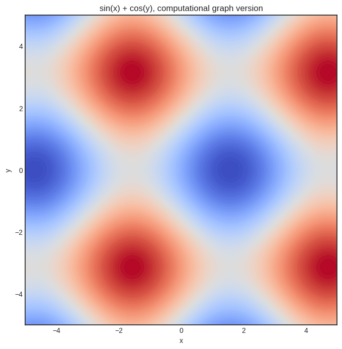
Just to convince you that it works, here’s the plot of our sin(x) + sin(y) function.
import matplotlib.pyplot as plt
import numpy as np


with plt.style.context("seaborn-v0_8-white"):
    plt.figure(figsize=(8, 8))

    res = 100
    x = np.linspace(-5, 5, res)
    y = np.linspace(-5, 5, res)
    xx, yy = np.meshgrid(x, y)

    zz = np.vectorize(lambda x, y: (sin(Scalar(x)) + cos(Scalar(y))).value)(xx, yy)

    plt.contourf(xx, yy, zz, levels=100, cmap='coolwarm_r')
    plt.xlabel('x')
    plt.ylabel('y')
    plt.title('sin(x) + cos(y), computational graph version')
    plt.show()
7.4. Linear regression as a computational graph#
We’re here to do machine learning, so how about implementing a linear regression model? First, the computational graph of \( ax + b \).
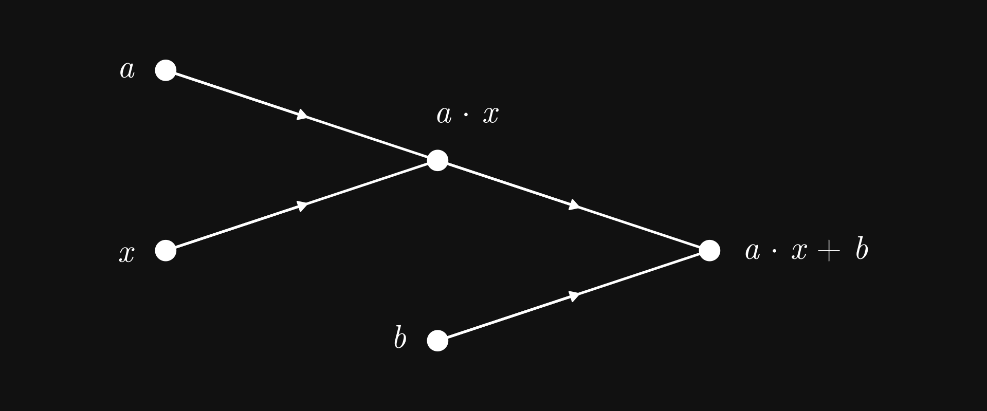
Fig. 7.4 Linear regression as a computational graph#
Nothing we haven’t seen before; in fact, structurally, it is the same as the graph of \( c (a + b) \). The only difference is the computations carried out by the nodes.
a = Scalar(3)
b = Scalar(-1)

def linear_regression(x: Scalar):
    return a*x + b
We can already glimpse the power of operator overloading: the function linear_regression is syntactically the same as the vanilla Python version, but this time, it can operate on our powerful Scalar objects. (Well, again, soon-to-be powerful.)
With this, we can even fully trace back the computations.
y = linear_regression(x=Scalar(0.5))

f"y = {y}, a*x = {y.prevs[0]}, b = {y.prevs[1]}, a = {y.prevs[0].prev.prevs[0]}, x = {y.prevs[0].prev.prevs[1]}"
'y = Scalar(0.5), a*x = Edge(prev=Scalar(1.5), local_grad=1), b = Edge(prev=Scalar(-1), local_grad=1), a = Edge(prev=Scalar(3), local_grad=0.5), x = Edge(prev=Scalar(0.5), local_grad=3)'
That’s cool, but why would we ever want to do that? It’s not clear at this point, but trust me on this, tracing the computations backward is a key tool in calculating derivatives effectively.
But why would we want to compute the derivative? Because we want to fit the model with gradient descent.
7.5. The backward pass#
To get a node’s derivative with respect to all preceding nodes, we use the famous backpropagation algorithm, implemented via the Scalar.backward method.
Let’s see it in action!
x, y = Scalar(1.2), Scalar(-6.9)
z = (sin(x) + cos(y))**2

z.backward()
Recall the mysterious Scalar.backwards_grad attribute? This is where z’s derivatives are stored! Upon calling z.backward(), the derivatives are calculated with respect to all preceding nodes, and then stored in the backwards_grad attribute.
Let’s see \( \frac{\partial z}{\partial x} \)!
x.backwards_grad
1.2666318116545192
What about \( \frac{\partial z}{\partial y} \)?
y.backwards_grad
2.021952608019056
As
we can check the correctness via Python’s built-in trigonometric functions from the math module.
from math import sin as sin_vanilla, cos as cos_vanilla

def z_grad(x, y):
    return (2 * cos_vanilla(x) * (sin_vanilla(x) + cos_vanilla(y)),
            -2 * sin_vanilla(y) * (sin_vanilla(x) + cos_vanilla(y)))

z_grad(x.value, y.value) == (x.backwards_grad, y.backwards_grad)
True
Yay!
Scalar is pretty simple to use; that was more or less all about it. In the next part, we’ll use computational graphs to train our first machine learning model: a linear regression. See you in the next chapter, where we will witness the true power of computational graphs!