8. Training neural networks

Before diving deep into the details of computational graphs, we’ll learn how to work with them. I know, you are probably eager to smash out your own backpropagation implementation, but it’s best to hold your horses. Mastering technical concepts happens in three stages:

1. understanding what you’re working with,

2. learning how to use it,

3. and finally, exploring how it works internally.

So, it’s time to put computational graphs to work. Let’s train some models!

Similarly to classical machine learning models like k-nearest neighbors or random forests, we want to build a convenient interface.

from mlfz.nn.scalar import Scalar


class Linear:
    def __init__(self):
        self.a = Scalar(1)
        self.b = Scalar(1)

    def __call__(self, *args, **kwargs):
        return self.forward(*args, **kwargs)

    def forward(self, x):
        return self.a * x + self.b
    
    def parameters(self):
        return {"a": self.a, "b": self.b}
    
    def gradient_update(self, lr):
        for _, p in self.parameters().items():
            p.value -= lr * p.backwards_grad

Let’s go through the methods one by one:

• Linear.forward, describes the computational graph that define the model,

• Linear.__call__ is a shortcut to Linear.forward,

• Linear.parameters, stores the model parameters in a dictionary,

• and Linear.gradient_update performs a step in gradient descent.

As you can see, there are several downsides of this implementation. For instance, Linear.parameters requires us to manually add all parameters one by one. Trust me, we’ll fix these early issues in due time.

For now, let’s see Linear in action!

linear = Linear()

linear.forward(2)

Scalar(3)

linear.parameters()

{'a': Scalar(1), 'b': Scalar(1)}

This is a good time to highlight that scalar operations work with vanilla number types, like integers, floats, whatever. It’s just for convenience, saving us from typing Scalar(...) all the time.

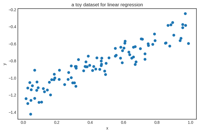
To train this simple model, we’ll generate a toy dataset from the target function \( h(x) = 0.8 x - 1.2 \).

from random import random, normalvariate


xs = [random() for _ in range(100)]
ys = [0.8*x - 1.2 + normalvariate(0, 0.1) for x in xs]

Show code cell source Hide code cell source

import matplotlib.pyplot as plt


with plt.style.context("seaborn-v0_8-white"):
    plt.figure(figsize=(8, 5))
    plt.scatter(xs, ys)
    plt.xlabel('x')
    plt.ylabel('y')
    plt.title('a toy dataset for linear regression')
    plt.show()

We’ll also need a loss function as well. Let’s go with the simplest one: the mean squared error, defined by the formula

\[ \mathrm{MSE}(\widehat{\mathbf{y}}, \mathbf{y}) = \frac{1}{N} \sum_{i=1}^{N} (\widehat{y}_i - y_i)^2, \]

where \( \widehat{\mathbf{y}} \in \mathbb{R}^N \) is the vector of predictions, while \( \mathbf{y} \in \mathbb{R}^N \) is the vector of ground truths.

from typing import List


def mean_squared_error(preds: List[Scalar], ys: List[Scalar]) -> Scalar:
    """
    Computes the mean squared error between the predictions and the ground truth.

    Args:
        preds (List[Scalar]): Predictions given by the model.
        ys (List[Scalar]): The ground truth.

    Returns:
        float: The mean squared error between the predictions and the ground truth.
    """
    return sum([(p - y) ** 2 for p, y in zip(preds, ys)]) / len(preds)

Again, notice that this is a vanilla Python function. Still, it can operate on our Scalar objects, turning computations into graphs.

preds = [linear(x) for x in xs]
mean_squared_error(preds, ys)

Scalar(5.28233493984566)

We already have everything ready to train our model with gradient descent!

n_steps = 100
lr = 0.2


for i in range(1, n_steps + 1):
    preds = [linear(x) for x in xs]
    l = mean_squared_error(preds, ys)
    l.backward()
    linear.gradient_update(lr=lr)
    
    if i == 1 or i % 10 == 0:
        print(f"step no. {i}, loss = {l.value}")

step no. 1, loss = 5.28233493984566
step no. 10, loss = 0.03469725326693804
step no. 20, loss = 0.02403273064267629
step no. 30, loss = 0.01773800899583241
step no. 40, loss = 0.014013106851795964
step no. 50, loss = 0.01180889563471076
step no. 60, loss = 0.0105045534260697
step no. 70, loss = 0.009732708793370475
step no. 80, loss = 0.009275969654607745
step no. 90, loss = 0.009005694223465355
step no. 100, loss = 0.008845758709996794

Here’s the result.

linear.parameters()

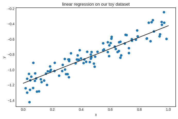
{'a': Scalar(0.7532478321623254), 'b': Scalar(-1.180013099282927)}

Looks good! The parameters seem close to the target function \( h(x) = 0.8x - 1.2 \). Here’s the plot.

Show code cell source Hide code cell source

with plt.style.context("seaborn-v0_8-white"):
    plt.figure(figsize=(8, 5))

    xs_plot = [0.01 * k for k in range(101)]
    ys_plot = [linear(x).value for x in xs_plot]
    plt.plot(xs_plot, ys_plot, c="k")

    plt.scatter(xs, ys)
    plt.xlabel('x')
    plt.ylabel('y')
    plt.title('linear regression on our toy dataset')
    plt.show()

8.1. Saving and loading parameters

Let’s go back to square one. What if we need to interrupt our training, to be continued later? Or load a pre-trained model?

This is an everyday circumstance in machine learning, especially with models of billions of parameters. Because of that, we’ll add a couple of methods to save and load weights.

from copy import deepcopy


class Linear(Linear):
    # ...

    def copy_parameters(self):
        return deepcopy(self.parameters())

    def load_parameters(self, params):
        for key, value in params.items():
            setattr(self, key, value)

linear = Linear()

linear.parameters()

{'a': Scalar(1), 'b': Scalar(1)}

Now, let’s load some new parameters.

linear.load_parameters({"a": Scalar(-1), "b": Scalar(-1)})

linear.parameters()

{'a': Scalar(-1), 'b': Scalar(-1)}

Keep in mind that in Python, Scalar objects are stored by reference, unlike, say, a Python float. This means that if you save the parameter dictionary and then use gradient descent to tune the parameters, your saved parameter dictionary will also change. Take a look.

print("using Model.parameters():")
linear = Linear()
p = linear.parameters()
print(f"before: p = {p}")

preds = [linear(x) for x in xs]
l = mean_squared_error(preds, ys)
l.backward()
linear.gradient_update(lr=10)
print(f"after: p = {p}")

using Model.parameters():
before: p = {'a': Scalar(1), 'b': Scalar(1)}
after: p = {'a': Scalar(-20.544558386909543), 'b': Scalar(-44.91606380836623)}

To avoid issues from this, we can use the Model.copy_parameters method.

print("using Model.copy_parameters():")
linear = Linear()
p = linear.copy_parameters()
print(f"before: p = {p}")

preds = [linear(x) for x in xs]
l = mean_squared_error(preds, ys)
l.backward()
linear.gradient_update(lr=10)
print(f"after: p = {p}")

using Model.copy_parameters():
before: p = {'a': Scalar(1), 'b': Scalar(1)}
after: p = {'a': Scalar(1), 'b': Scalar(1)}

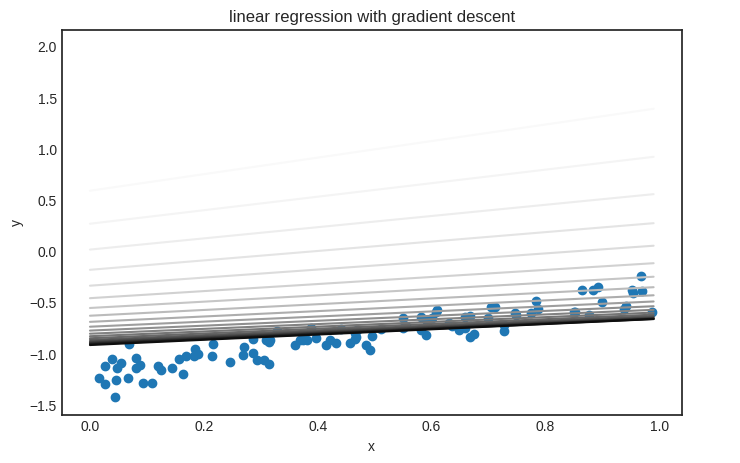
Parameter saving and loading are useful if you want to visualize the model’s state during training. Here’s an example demonstrating how gradient descent fits a linear regression model.

linear = Linear()

n_steps = 200
lr = 0.01

parameter_list = [linear.copy_parameters()]

for _ in range(n_steps):
    preds = [linear(x) for x in xs]
    l = mean_squared_error(preds, ys)
    l.backward()
    linear.gradient_update(lr)
    parameter_list.append(linear.copy_parameters())

Show code cell source Hide code cell source

from matplotlib import colormaps

color_map = colormaps['Greys']

with plt.style.context('seaborn-v0_8-white'):
    plt.figure(figsize=(8, 5))
    plt.scatter(xs, ys)

    xs_plot = [k*0.01 for k in range(100)]

    trimmed_parameter_list = parameter_list[::10]
    for i, params in enumerate(trimmed_parameter_list):
        color = color_map(i / len(trimmed_parameter_list))
        linear.load_parameters(params)
        ys_plot = [linear(x).value for x in xs_plot]
        plt.plot(xs_plot, ys_plot, color=color)

    plt.title("linear regression with gradient descent")
    plt.xlabel("x")
    plt.ylabel("y")
    plt.legend(bbox_to_anchor=(1.05, 0.0), loc='lower left')
    plt.show()

/tmp/ipykernel_59726/2321412048.py:21: UserWarning: No artists with labels found to put in legend.  Note that artists whose label start with an underscore are ignored when legend() is called with no argument.
  plt.legend(bbox_to_anchor=(1.05, 0.0), loc='lower left')

It’s time to see an actual neural network!

8.2. Building a neural network

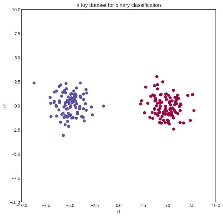
We start with a simple binary classification problem to demonstrate how neural networks work. Here’s our (generated) dataset of two blue and red classes encoded with 0 and 1.

import random
import matplotlib.pyplot as plt


xs = [(random.normalvariate(0, 1) - 5 , random.normalvariate(0, 1)) for _ in range(100)] \
    + [(random.normalvariate(0, 1) + 5 , random.normalvariate(0, 1)) for _ in range(100)]
ys = [1 for _ in range(100)] + [0 for _ in range(100)]

Show code cell source Hide code cell source

with plt.style.context("seaborn-v0_8-white"):
    plt.figure(figsize=(8, 8))
    plt.xlim([-10, 10])
    plt.ylim([-10, 10])
    plt.scatter([x[0] for x in xs], [x[1] for x in xs], c=ys, cmap=plt.cm.Spectral)
    plt.title("a toy dataset for binary classification")
    plt.xlabel("x1")
    plt.ylabel("x2")
    plt.show()

We’ll start with the simplest neural network: zero hidden layers and sigmoid activation. This is also known as logistic regression. Here we go:

from mlfz.nn.scalar import Scalar, sigmoid, binary_cross_entropy


class ZeroLayerNetwork:
    def __init__(self):
        self.a1 = Scalar(1)
        self.a2 = Scalar(1)
        self.b = Scalar(1)

    def __call__(self, *args, **kwargs):
        return self.forward(*args, **kwargs)

    def forward(self, x):
        x1, x2 = x
        return sigmoid(self.a1 * x1 + self.a2 * x2 + self.b)
    
    def parameters(self):
        return {"a1": self.a1, "a2": self.a2, "b": self.b}
    
    def gradient_update(self, lr):
        for _, p in self.parameters().items():
            p.value -= lr * p.backwards_grad

model = ZeroLayerNetwork()

Show code cell source Hide code cell source

import numpy as np


def visualize_model(model, xs, ys, res=100, xrange=(-10, 10), yrange=(-10, 10)):
    with plt.style.context("seaborn-v0_8-white"):
        plt.figure(figsize=(8, 8))
        
        res = 100
        x = np.linspace(xrange[0], xrange[1], res)
        y = np.linspace(yrange[0], yrange[1], res)
        xx, yy = np.meshgrid(x, y)
        
        zz = np.vectorize(lambda x, y: model((x, y)).value)(xx, yy)

        # plot the decision boundary
        plt.contourf(xx, yy, zz, levels=100, cmap='coolwarm_r', alpha=0.4)
        plt.xlabel('x')
        plt.ylabel('y')
        plt.title('the decision boundary of our model')
        
        # plot the data
        plt.scatter([x[0] for x in xs], [x[1] for x in xs], c=ys, cmap=plt.cm.Spectral, zorder=10)
        plt.show()


visualize_model(model, xs, ys)

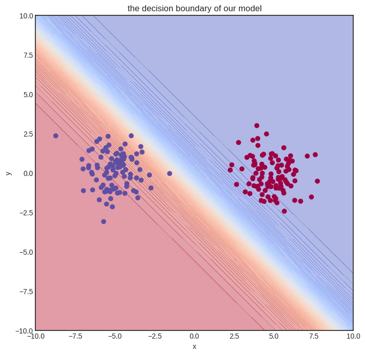
The initial model gets nothing right, so let’s train it!

n_steps = 100
lr = 0.1

for i in range(1, n_steps + 1):
    preds = [model(x) for x in xs]
    l = binary_cross_entropy(preds, ys)
    l.backward()
    model.gradient_update(lr)

    if i == 1 or i % 10 == 0:
        print(f"step no. {i}, loss = {l.value}")

step no. 1, loss = 4.800382749384406
step no. 10, loss = 0.10238898440442779
step no. 20, loss = 0.04344827744067521
step no. 30, loss = 0.02753314388111004
step no. 40, loss = 0.02018260303976357
step no. 50, loss = 0.015963508691694668
step no. 60, loss = 0.013229508717900667
step no. 70, loss = 0.011314315687163366
step no. 80, loss = 0.009897767570211082
step no. 90, loss = 0.008807185063395298
step no. 100, loss = 0.007941316866188004

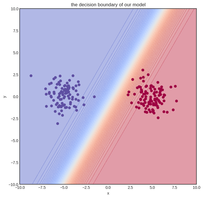
Here’s how the model performs after training. Judging from the loss values, it’s pretty good.

Show code cell source Hide code cell source

visualize_model(model, xs, ys)

Solving a simple problem like that is no big deal. Can we handle more complex datasets?

8.3. A multi-layer network

Here’s a spiral-like dataset with classes intertwined into each other. (Feel free to skip the generating code; it’s irrelevant to our purposes. Hell, I even confess that it was made by ChatGPT.)

Show code cell source Hide code cell source

import math


def generate_spiral_dataset(n_points, noise=0.5, twist=380):
    random_points = [math.sqrt(random.random()) * twist * 2 * math.pi/360 for _ in range(n_points)]

    class_1 = [(-math.cos(p) * p + random.random()*noise, math.sin(p) * p + random.random()*noise) for p in random_points]
    class_2 = [(math.cos(p) * p + random.random()*noise, -math.sin(p) * p + random.random()*noise) for p in random_points]

    xs = class_1 + class_2
    ys = [0 for _ in class_1] + [1 for _ in class_2]
    
    return xs, ys

xs, ys = generate_spiral_dataset(200, noise=2)

Show code cell source Hide code cell source

with plt.style.context("seaborn-v0_8-white"):
    plt.figure(figsize=(8, 8))
    plt.scatter([x[0] for x in xs], [x[1] for x in xs], c=ys, cmap=plt.cm.Spectral)
    plt.show()

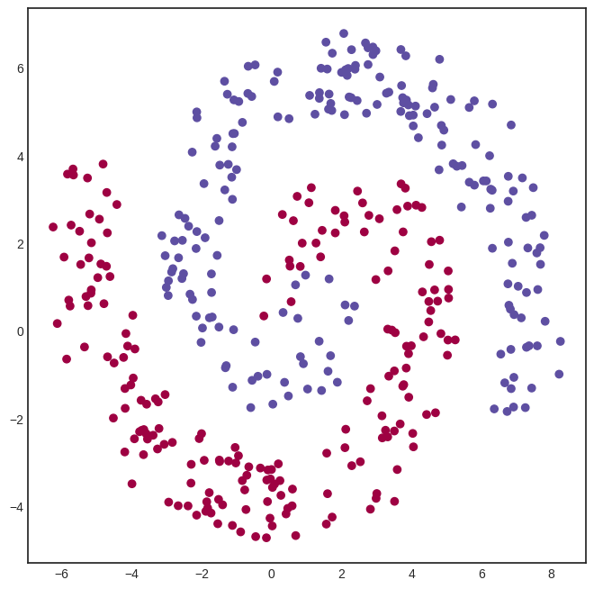
A logistic regression model won’t cut it this time. To solve this classification problem, we need a hidden layer. Here’s a model with a hidden layer of eight neurons, connected via the

\[ \mathrm{tanh}(x) = \frac{e^{2x} - 1}{e^{2x} + 1} \]

activation function.

from mlfz.nn.scalar import tanh
from itertools import product
from typing import Tuple


class OneLayerNetwork:
    def __init__(self):
        self.A = [[Scalar.from_random() for j in range(16)]
                  for i in range (2)]
        self.B = [Scalar.from_random() for i in range(16)]
  
    def __call__(self, *args, **kwargs):
        return self.forward(*args, **kwargs)
    
    def forward(self, x: Tuple[Scalar]):
        """
        x: a tuple of two Scalars
        """
        fs = [sum([self.A[i][j] * x[i] for i in range(2)]) for j in range(16)]
        fs_relu = [tanh(f) for f in fs]
        gs = sum([self.B[i] * fs_relu[i] for i in range(16)])
        return sigmoid(gs)

    def parameters(self):
        A_dict = {f"a{i}{j}": self.A[i][j] for i, j in product(range(2), range(16))}
        B_dict = {f"b{i}": self.B[i] for i in range(16)}
        return {**A_dict, **B_dict}
    
    def gradient_update(self, lr):
        for _, p in self.parameters().items():
            p.value -= lr * p.backwards_grad

We can already see one of the glaring flaws of our Scalar implementation of computational graphs: the inability to write vectorized code. For instance, the expression

fs = [sum([self.A[i][j] * x[i] for i in range(2)]) for j in range(4)]

is simply the matrix product of the input x and the \( 2 \times 4 \) parameter matrix A.

We’ll deal with vectorization later with the Tensor class, but let’s stick to the vanilla version for now. Here’s our model.

model = OneLayerNetwork()

And here’s how the untrained model looks.

Show code cell source Hide code cell source

visualize_model(model, xs, ys)

Let’s train it! We’ll need quite some more steps. To spice things up, we’ll also use a simple learning rate tuning: lr=1 for the first hundred gradient descent steps, lr=0.5 for the second hundred, and lr=0.1 after.

def lr_fn(i):
    if i < 100:
        return 1
    elif i < 400:
        return 0.5
    else:
        return 0.1

n_steps = 1000


for i in range(1, n_steps + 1):
    preds = [model(x) for x in xs]
    l = binary_cross_entropy(preds, ys)
    l.backward()
    model.gradient_update(lr_fn(i))

    if i == 1 or i % 100 == 0:
        print(f"step no. {i}, loss = {l.value}")

step no. 1, loss = 1.5035309829960366
step no. 100, loss = 0.4959981139585014
step no. 200, loss = 0.4305200947399042
step no. 300, loss = 0.42887467278688374
step no. 400, loss = 0.42874093217118664
step no. 500, loss = 0.37735450915599295
step no. 600, loss = 0.3725885659861823
step no. 700, loss = 0.36955964143639675
step no. 800, loss = 0.3673377754955526
step no. 900, loss = 0.3655672435159357
step no. 1000, loss = 0.364083449533418

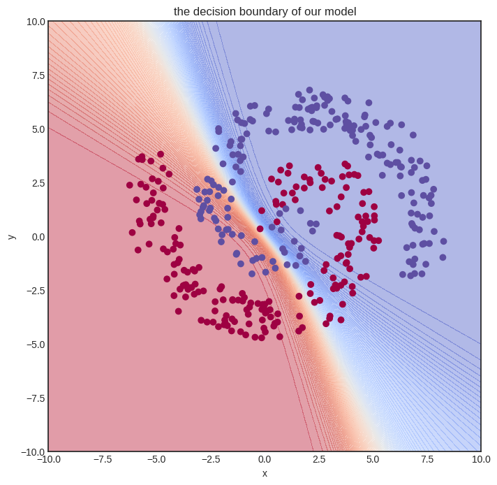
This training took a while to execute on my Lenovo Thinkpad (the machine on thich I am writing this book). Again, this is the consequence of non-vectorized code. Is the model any good? Let’s see.

Show code cell source Hide code cell source

visualize_model(model, xs, ys)

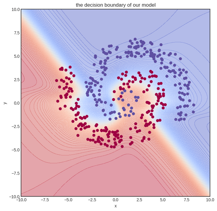
Not perfect at all, but we can already see that the decision boundary is starting to conform to the data. We need a more expressive model and more training iterations. This foreshadows the need for more effective code, which we’ll bring to fruition with vectorization.

But let’s not get ahead of ourselves and see how Scalar works on the inside! Trust me on this: understanding plain scalar-valued computational graphs is paramount to building hyper-fast vectorized ones. We dial up the difficulty one notch at a time, and right now, the next step is digging deep into the forward pass.