2. The taxonomy of machine learning paradigms#
To look behind the curtain of machine learning algorithms, we have to precisely formulate the problems that we deal with. Three important parameters determine a machine learning paradigm: the input, the output, and the training data.
All machine learning tasks boil down to finding a model that provides additional insight into the data, i.e., a function \( f \) that transforms the input \( x \) into the useful representation \( y \). This can be a prediction, an action to take, a high-level feature representation, and many more. We’ll learn about all of them.
Mathematically speaking, the basic machine learning setup consists of:
a dataset \( \mathcal{D} \),
a function \( f \) that describes the true relation between the input and the output,
and a parametric model \( h \) — also called a hypothesis — that serves as our estimation of \( f \).
Remark 2.1 (Common abuses of machine learning notation.)
Note that although the function \( f \) only depends on the input \( x \), the parametric model \( h \) also depends on the parameters and the training dataset.
Thus, it is customary to write \( h(x) \) as \( h(x; w, \mathcal{D}) \), where \( w \) represents the parameters, and \( \mathcal{D} \) is our training dataset.
This dependence is often omitted, but keep in mind that it’s always there.
We make no restrictions about how the model \( \hat{f} \) is constructed. It can be a deterministic function like \( h(x) = -13.2 x^2 + 0.92 x + 3.0 \) or a probability distribution \( h(x) = P(Y = y \mid X = x) \). Models have all kinds of families like generative, discriminative, and more. We’ll talk about them in detail; in fact, models will be the focal points of the next few chapters.
First, let’s focus on the paradigms themselves. There are four major ones:
supervised learning,
unsupervised learning,
semi-supervised learning,
and reinforcement learning.
What are these?
2.1. Supervised learning#
The most common paradigm is supervised learning. There, we have inputs \( x_i \) and ground truth labels \( y_i \) that form our training dataset
Although the labels can be anything like numbers or text, they are all available for us. The goal is to construct a function that models the relationship between the input \( x \) and the target variable \( y \).
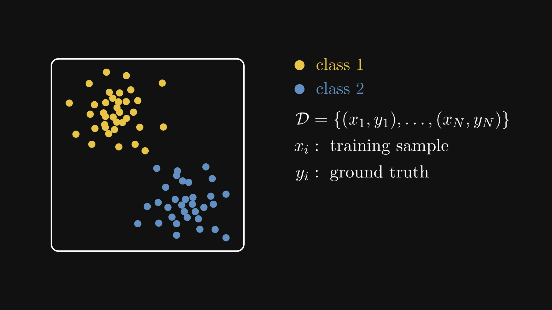
Fig. 2.1 A supervised learning dataset.#
Here are the typical unsupervised learning problems.
Example 1. You are building the revolutionary “Hot Dog or Not” mobile app, aiming to determine if the phone’s camera is pointed towards a hot dog or not, That is, your input is a matrix \( X \in \mathbb{R}^{n \times m} \) (where \( n \) and \( m \) represent the dimensions of the image), and the output is a categorical variable \( y \in \{ \text{not dog}, \text{not hot dog} \} \).
Example 2. You are a quant, tasked to predict the future price of Apple stock, based on its price history last week. That is, the input is a vector \( \mathbf{x} = (x_1, \dots, x_7) \in \mathbb{R}^7 \), and the output is a real number \( y \in \mathbb{R} \).
Example 3. You are a machine learning engineer at Tesla, working on identifying obstacles and objects shown on the built-in cameras. That is, given a \( 1024 \times 768 \) image, your job is to list all of its objects and their bounding boxes. Once again, the input is a matrix \( X \in \mathbb{R}^{1024 \times 768} \), and the output is a set
where \( (x_{i 1}, x_{i 2}, x_{i 3}, x_{i 4}) \in \mathbb{R}^k \) and \( y_i \) is an element of the possible objects on the image. (Note that the size of the output set can vary from image to image.)
As you can see, the tasks are quite diverse. It’s important to note that it’s not the problem itself that makes it supervised, but the availability of ground truth.
When the ground truth consists of categorical labels, we are talking about classification. (Such as the hot dog classification and the object detection example above.) If the target variable is a real number, this is regression. (Like our stock market prediction example.)
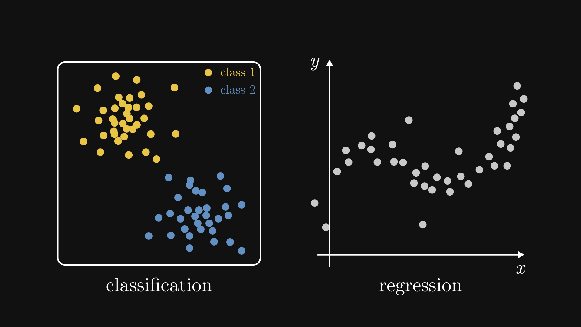
Fig. 2.2 Classification vs. regression.#
2.2. Unsupervised learning#
Although supervised learning is powerful, we don’t always have labeled data. For instance, payment providers have a record of millions of credit card transactions. How do they filter out the fraudulent ones? Labeled data is very hard to generate in this scenario. Unsupervised learning aims to overcome this problem.
The setup is simple: as opposed to supervised learning, we only have the inputs \( x_i \), so our dataset is
In this case, our job is to identify patterns that can help us infer the class labels. However, not only we do not have ground truth, we also don’t know what the possible classes are. This is the main challenge of unsupervised learning.
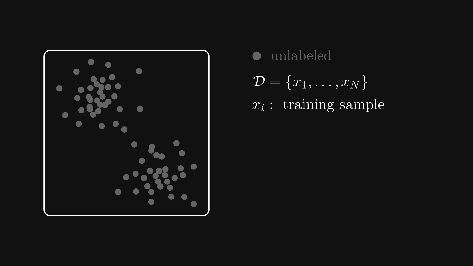
Fig. 2.3 An unsupervised learning dataset.#
Examples, examples, examples.
Example 1. You are the growth hacker of an e-commerce startup, aiming to improve ad targeting via customer segmentation. There are two challenges: 1) customers seldom identify and report themselves as belonging to a particular segment, and 2) the segments are not even well-defined. This task is called clustering.
Formally, the input data consists of a sequence of vectors \( {x_1, x_2, \dots, x_N} \), and the expected output is the sequence of labels \( {y_1, y_2, \dots, y_N} \), where \( y_i \in \{ 1, 2, \dots, l \} \) is the label corresponding to the input \( x_i \).
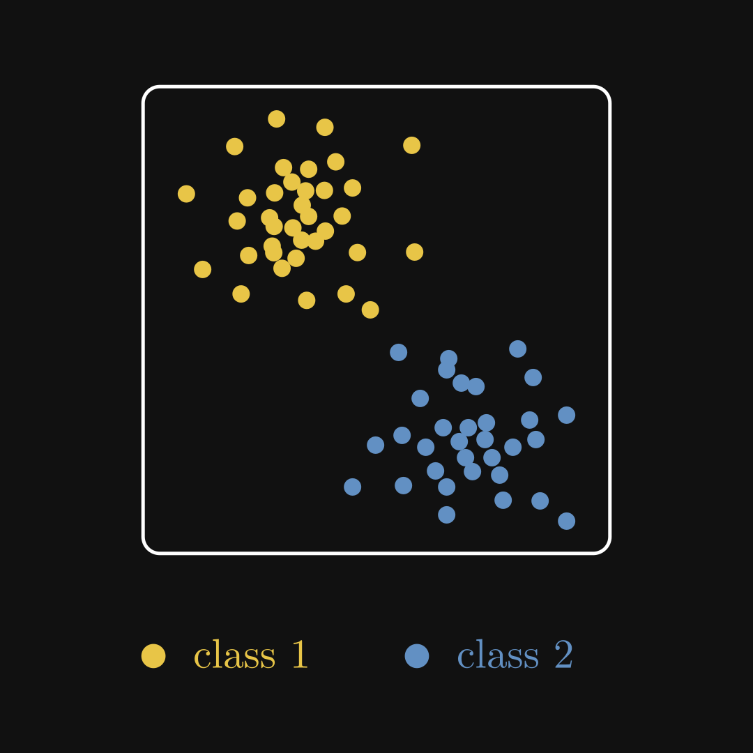
Fig. 2.4 The output of a clustering algorithm.#
Example 2. You are a cybersecurity consultant, tasked by an enterprise to detect suspicious activity on the servers. You have a ton of log files, but since hackers usually don’t introduce themselves to you and show the exact steps they took, you don’t have any labels at all. As malicious activities are extremely rare, you are looking for needles in a haystack. This is the task of anomaly detection.
The input and the expected output are similar to clustering: a sequence of vectors \( {x_1, x_2, \dots, x_N} \) as inputs, and a sequence of labels \( {y_1, y_2, \dots, y_N} \) as outputs. This time, however, \( y_i \) is either zero or one. Zero for business-as-usual, and one for anomalous activities. The main difference from clustering is that the vast majority of labels will belong to the business-as-usual class.
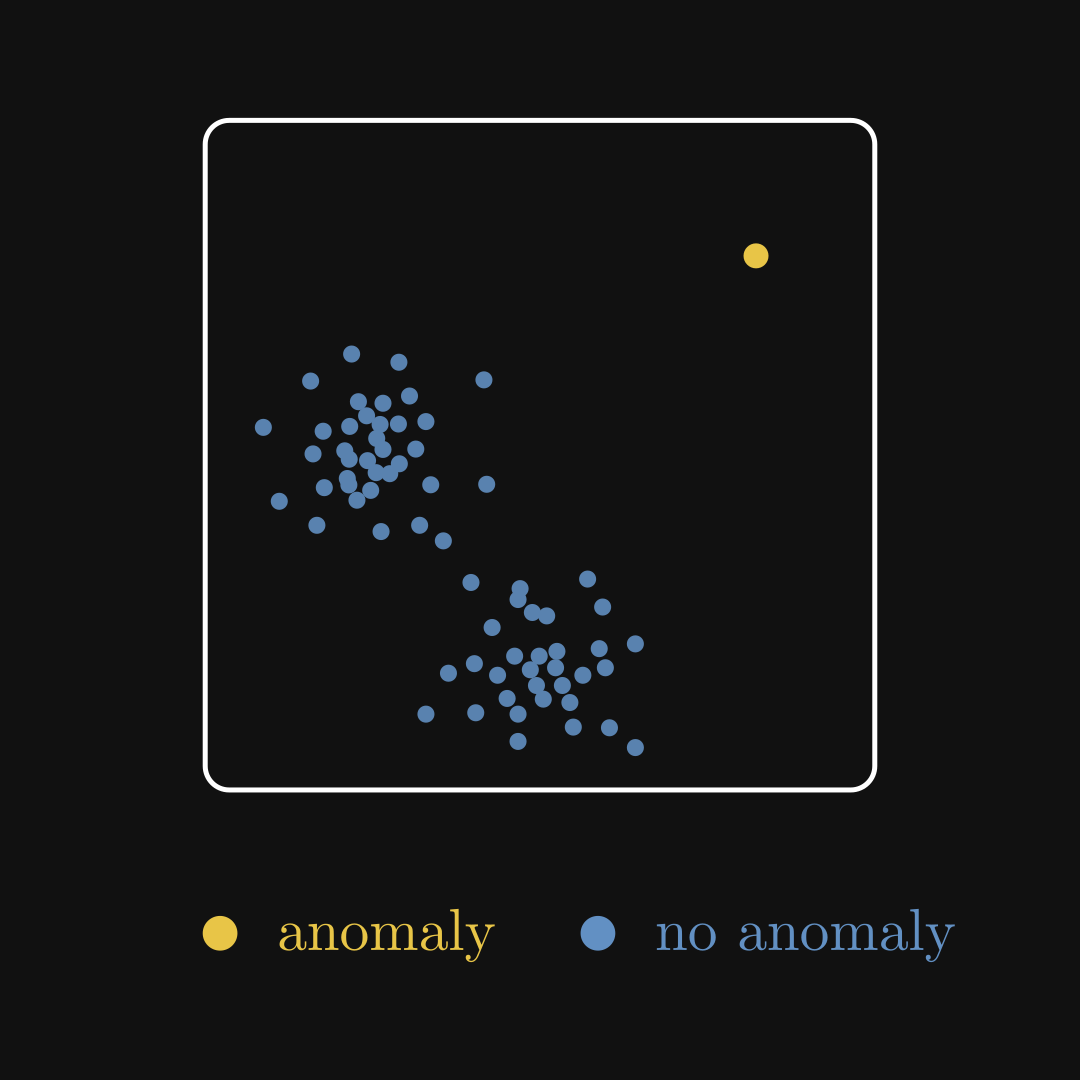
Fig. 2.5 Anomaly detection.#
Example 3. You are a molecular biologist, aiming to characterize cells based on genomic data: for each cell, you have an \( n \)-dimensional vector \( x_i \in \mathbb{R}^n \) that describes its molecular composition. The catch is, \( n \) is very large, and the vast majority of features do not contribute to the phenotype. (That is, they are just noise.) Thus, you need to find a lower-dimensional representation \( y_i \in \mathbb{R}^m \) that preserves the structure of the data but eliminates the noise and redundancies. (Preferably, \( m \) is a few orders of magnitude smaller than \( n \).) This is dimensionality reduction.
In general, clustering aims to group the data points into classes based on their features; anomaly detection finds rare instances in the data; dimensionality reduction transforms the dataset into a lower-dimension representation with more expressive features. When successful, dimensionality reduction can make clustering and anomaly detection easier, so combining them can be particularly effective.
If we cut down the last layer of a neural network, we obtain a really strong dimensionality reduction tool. Neural networks learn a high-level feature representation of the data based on the training labels. The last layer is often a simple linear classifier, but the features provided by the rest of the network are so descriptive that even this can perform exceptionally well. Note that a neural network often learns the features from data, so it is not always applicable to the case of unsupervised learning. However, the point is clear: a good dimensionality reduction is often key to good performance.
2.3. Semi-supervised learning#
Having no labels and having all the labels are the two ends of the same spectrum. This is usually not the case in practice.
Getting raw data is much faster and cheaper than labelling. However, annotating a subset of them is perfectly feasible though, so why not take advantage of it? This is called semi-supervised learning. In this scenario, our dataset is a hybrid of the previous two:
Typically, unlabeled data is much more abundant than labeled.
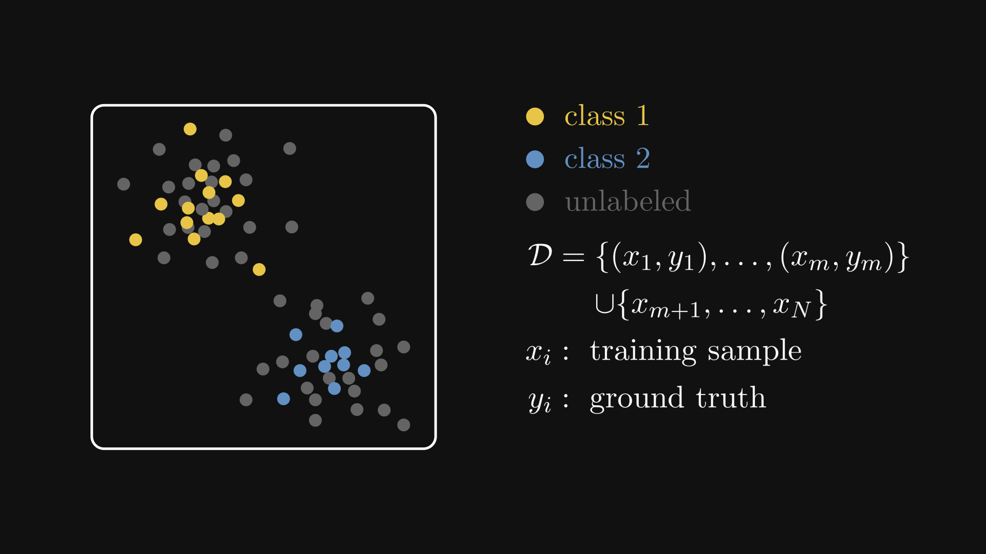
Fig. 2.6 A semi-supervised learning dataset.#
Here are some examples.
Example 1. You are the chief machine learning engineer at a biomedical startup, aiming to revolutionize skin cancer diagnostics via computer-vision driven tools. Your main product is an image classifier, able to diagnose skin cancer based on a single image of the skin tissue in question.
Images are quick and cheap to obtain, but labeling them requires an expert dermatologist. As expert time is expensive, you only have a couple thousand annotated images; on the other hand, you have millions of unlabelled ones. A possible labeling approach is the following.
Train a baseline model using the available data.
Determine which unlabelled images would increase the model’s performance the most.
Have an expert annotate the selected images.
Retrain the model and repeat the procedure.
This is called active learning.
Example 2. You are the chief machine learning engineer of a finance startup, putting AI on the blockchain providing alternative data to trading firms by turning financial news into feature vectors. (Perhaps my examples indicate that deep down, I wish to be the chief machine learning engineer of a startup. Well, maybe after I finish my book.)
Sentiment classification is a major part of your pipeline, but there is a snag: financial news are pouring like the rain, and you just don’t have the capacity to label at all. What’s worse is that the data keeps on changing: new technical terms pop up every day, companies come and go, and the world moves much faster than you can keep up with it. One possible solution is weak supervision: define weak labelling functions based on heuristics, classifying positive or negative sentiments based on the presence of a different keywords, like “terrible”, “powerful”, “recommended”, etc. These are often not accurate enough to base any serious prediction on them, but combined together, they can be used to train a significantly better model.
For comparison, here are the supervised, unsupervised, and semi-supervised datasets on a single image.
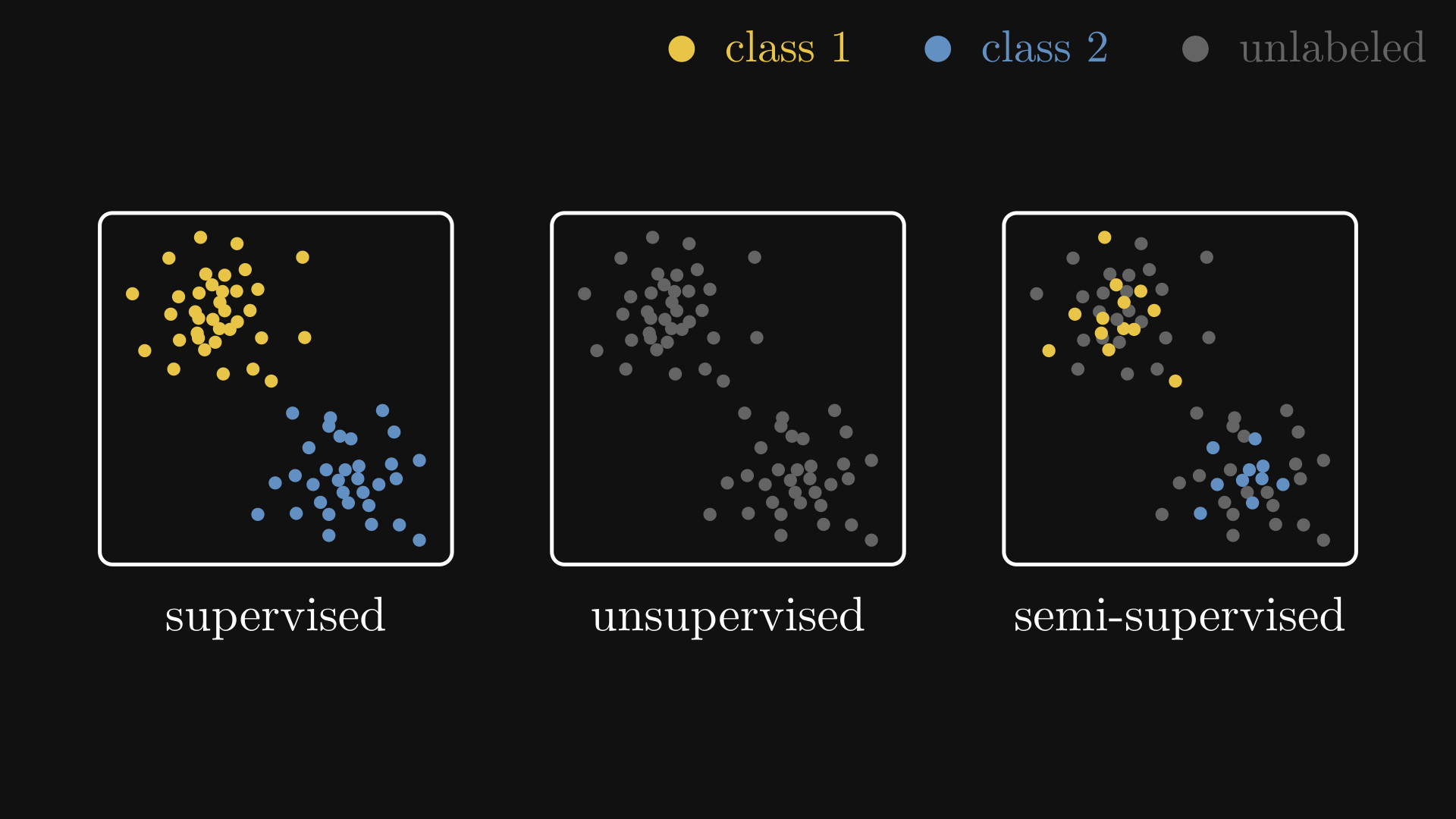
Fig. 2.7 Semi, un-, and supervised learning datasets.#
2.4. Reinforcement learning#
Some scenarios don’t fit any of the supervised, unsupervised, or semi-supervised cases. For instance, consider playing a game of Go. Can you teach a machine to play and eventually master it? Sure, you can generate data by recording games and training a supervised learning algorithm on them, but that would only teach the model to play like the humans who generated the dataset. Is this how Google’s AlphaGo beat the best Go player in the world? No.
AlphaGo used reinforcement learning. Instead of learning to play by looking at someone else, reinforcement learning allows models to learn by playing the game themselves. In its world, there is a model-controlled agent that applies certain actions in an environment, changing its state and receiving a reward when the action is appropriate. Based on the reward and the new state, the model learns to adjust the actions to maximize reward.
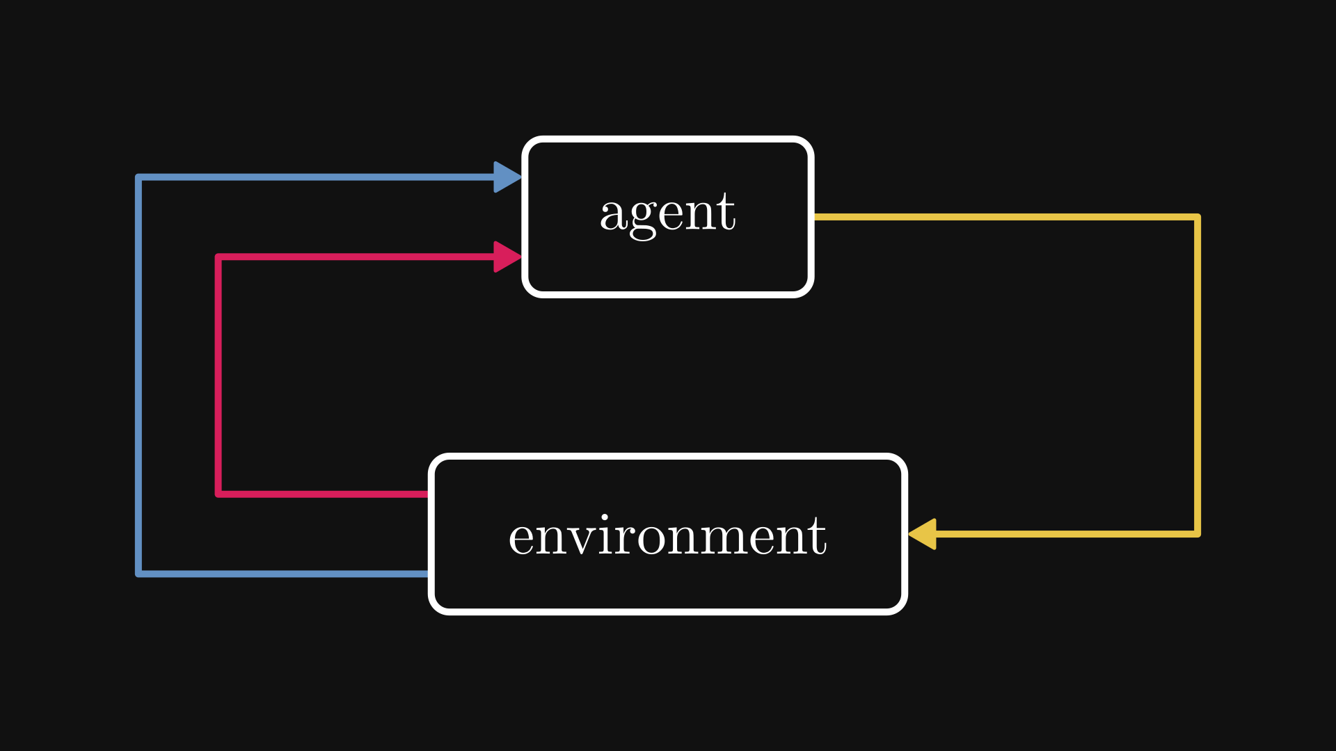
Fig. 2.8 The reinforcement learning worldview.#
At first glance, reinforcement learning might feel supervised: the training data is also of the form \( ((x_i, s_i), y_i) \), where \( x_i \) is the action, \( s_i \) is the state of the system, and \( y_i \) is the reward.
There are two key differences. First, the reward is not immediately available. Say, think of chess. Every move is considered an action, but the reward can only be determined at the end of the game.
Second, is that while supervised learning strives to engineer training datasets that are similar in distribution to the underlying data-generating process, this is not true for reinforcement learning. If our goal is to win a game, we don’t want to explore the losing moves, just the winning ones. Reinforcement learning is a balance of exploration and exploitation, while supervised learning goes full exploration.
Although reinforcement learning is an exciting field, we are not going to discuss it further. If you are interested in learning more, check out Deep Reinforcement Learning: Pong from Pixels by Andrej Karpathy, which is a great read.