Linear regression

3. Linear regression#

Now that we understand what machine learning is, we are ready to implement its “Hello, World!”: linear regression.

However, contrary to the “Hello, World!” program, linear regression is not only a warming-up exercise; it is the most important machine learning model. Besides teaching us the fundamentals, linear regression is everywhere. For instance, linear models are the soul of neural networks.

In the following, we’ll learn everything about this simple model. And I do mean everything: linear regression has quite a few different faces. We’ll take a look at all of them, and implement our own custom linear regressor from scratch.

3.1. The base model#

Let’s consider a basic regression problem: we have

two variables \( x \) and \( y \), (for example, representing the square footage and the price of a real estate; or the study hours and the final test score of a student)
and a set of observations \( \mathcal{D} = \{ (x_i, y_i): i = 1, \dots, n \} \).

Our goal is to predict \( y \) from \( x \); that is, the dependent variable from the independent variable. In other words, we are looking for a function \( h: \mathbb{R} \to \mathbb{R} \) that fits our observations as good as possible.

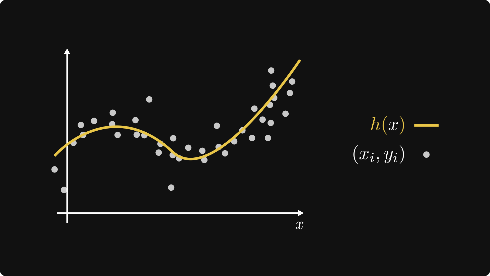
../_images/regression.png — Fig. 3.1 A regression problem.#

There are two key design choices that determine our machine learning model:

the family of functions we pick our \( h \) from (that is, our hypothesis space),
and the measure of fit. (That is, our loss function.)

Linear regression represents the simplest possible choices: we are looking for a function of the form \( h(x; a, b) = ax + b \), where \( a, b \in \mathbb{R} \) are two real parameters, and we measure the fit by the mean-squared error

\[ \mathrm{MSE}(h, \mathcal{D}) = \frac{1}{n} \sum_{i=1}^{n} \big( h(x_i; a, b) - y_i \big)^2. \]

Remark 3.1 (From abstract to concrete.)

When going from abstract to concrete, i.e. from theory to implementation, we’ll often perform sleight of hands like writing \( \mathrm{MSE}(a, b, \mathcal{D}) \) instead of \( \mathrm{MSE}(h, \mathcal{D}) \). We can do this without skipping a beat, as \( h(x) = ax + b \) can be thought of as a function of the parameters \( a \) and \( b \). Keep this in mind, as we’ll do this quite frequently.

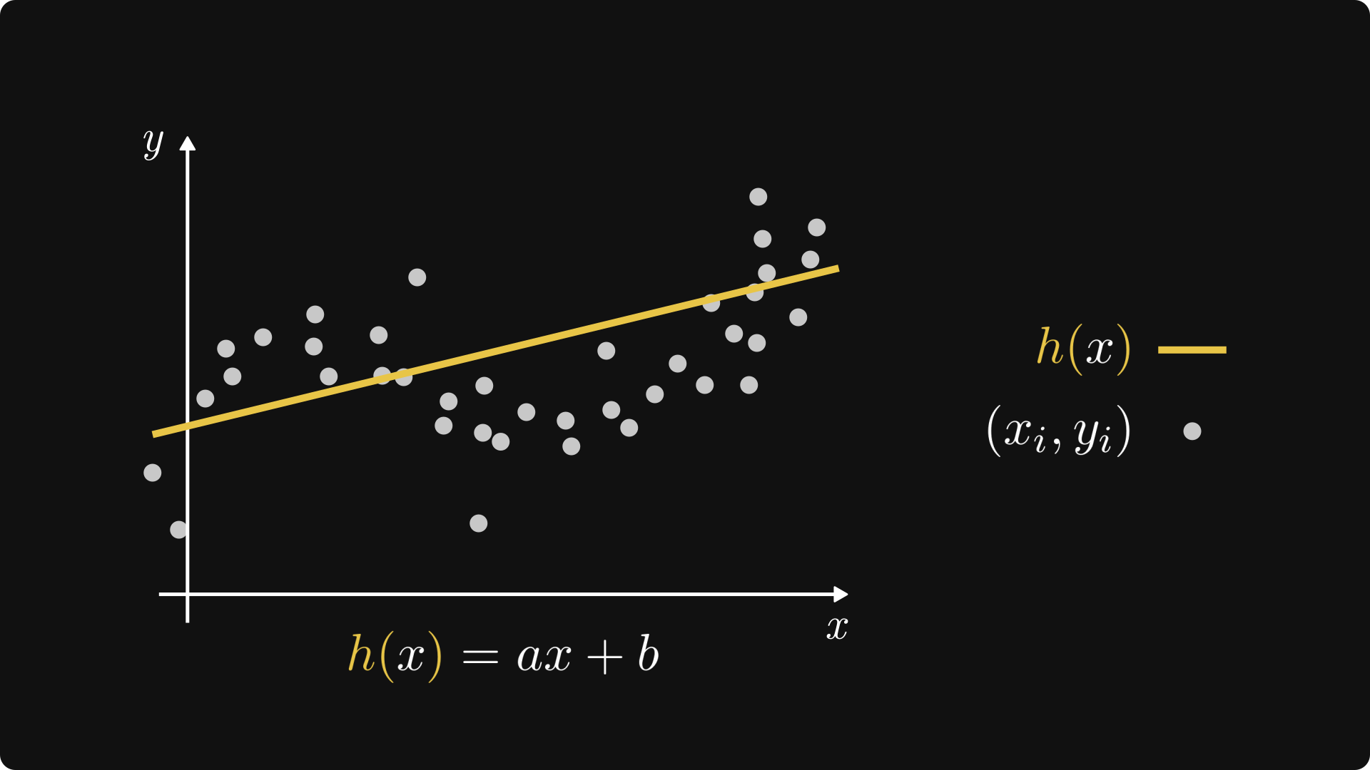
../_images/linear-regression.png — Fig. 3.2 Linear regression.#

For notational simplicity, we’ll most often omit the dependence of the parameters; that is, write \( h(x) \) in place of \( h(x; a, b) \). When it adds to the discussion, we’ll be really explicit and include the parameters as well.

Remark 3.2 (From concrete to abstract.)

To be really pedantic about our choices, we define the hypothesis space by

\[ \mathcal{H} = \{ h(x; a, b) = ax + b: a, b \in \mathbb{R} \}, \]

which is a set of functions; and we define the measure of fit \( L: \mathcal{H} \to \mathbb{R} \) by

\[ L(h) = \mathrm{MSE}(h, \mathcal{D}) = \frac{1}{n} \sum_{i=1}^{n} \big( h(x_i; a, b) - y_i \big)^2. \]

We can turn up the mathematical pedantry ad infinitum, but that’s not why we are here. I promise you to keep these to a bare minimum, and add them only when necesary.

Both of these components have a simple visual interpretation. For one, functions in the form of \( h(x) = ax + b \) represent a straight line, hence the name linear regression.

Remark 3.3 (Linear vs. affine functions.)

If we want to be mathematically precise, the function \( h(x) = ax + b \) is not linear. We say that a function \( f(x) \) is linear if \( f(\alpha x + \beta y) = \alpha f(x) + \beta f(y) \) holds for all \( \alpha \), \( \beta \), \( x \), and \( y \). This is does not hold for \( h(x) = ax + b \).

However, \( ax + b \) is not that far from an affine function. Geometrically speaking, the \( ax \) part is simply a stretching, which is a linear transformation. However, the \( \cdot + b \) part represent a translation, and overall, \( ax + b \) maps lines to lines. (Which makes more sense in higher dimensions, but still valid in one variable as well.)

Hence, functions of the form \( ax + b \) are called affine.

Geometrically, \( a \) is the slope of the line, while \( b \) shows where our line intersects the \( y \) axis. \( a \) is the regression coefficient, while \( b \) is the intercept of the linear model.

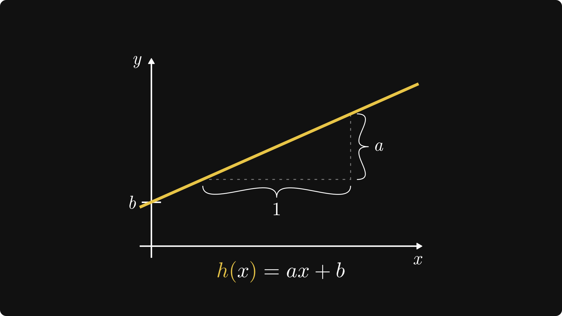
../_images/intercept-and-coefficient.png — Fig. 3.3 The intercept and the regression coefficient.#

Moreover, for any given observation \( (x_i, y_i) \), the quantity \( (h(x_i) - y_i)^2 \) is the squared distance between \( h(x_i) \) (that is, our prediction for \( x_i \)) and \( y_i \) (that is, the ground truth). The mean-squared error is simply the average of such squared distances.

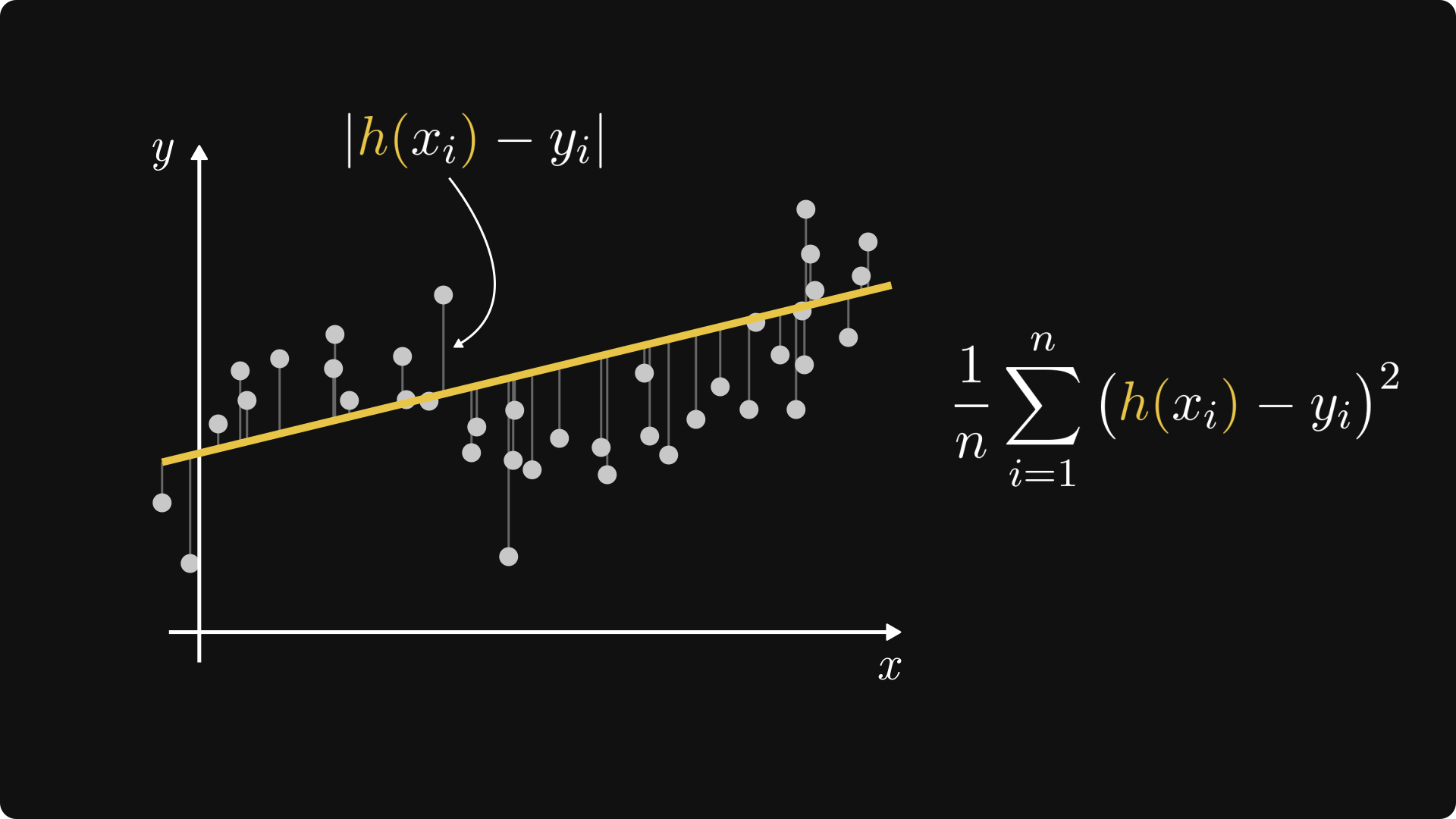
../_images/mse.png — Fig. 3.4 The mean-squared error.#

3.2. Finding the best fit with gradient descent#

Now that we have our model and our loss function, the question is this: how do we find the best fit?

Mathematically speaking, the problem is to minimize the loss function

\[ L(a, b) = \frac{1}{n} \sum_{i=1}^{n} (a x_i + b - y_i)^2, \]

that is, our parameter estimates are

\[ \hat{a}, \hat{b} = \arg \min_{a, b \in \mathbb{R}} L(a, b). \]

How to find them? With gradient descent. Let’s recap before we implement our own from scratch. Introducing the vectorized notation \( \mathbf{w} = (a, b)\), gradient descent consists of

selecting a set of initial parameters \( \mathbf{w}_0 \),
then iterating \( \mathbf{w}_{k+1} = \mathbf{w}_k - \alpha \nabla L(\mathbf{w}_k) \) until convergence,

where \( \alpha > 0 \) is the so-called learning rate, and \( \nabla L(\mathbf{w}) \) is the gradient of \( L \) with respect to \( \mathbf{w} \).

Regarding \( \nabla L \), we have

(3.1)#\[\begin{split} \begin{align*} \frac{\partial L}{\partial a} &= \frac{\partial}{\partial a} \bigg[ \frac{1}{n} \sum_{i=1}^{n} (a x_i + b - y_i)^2 \bigg] \\ &= \frac{1}{n} \sum_{i=1}^{n} \frac{\partial}{\partial a} (a x_i + b - y_i)^2 \\ &= \frac{1}{n} \sum_{i=1}^{n} 2 x_i (a x_i + b - y_i), \end{align*} \end{split}\]

and similarly,

(3.2)#\[ \begin{align*} \frac{\partial L}{\partial b} = \frac{1}{n} \sum_{i=1}^{n} 2(a x_i + b - y_i). \end{align*} \]

Coding time.

import numpy as np
import matplotlib.pyplot as plt

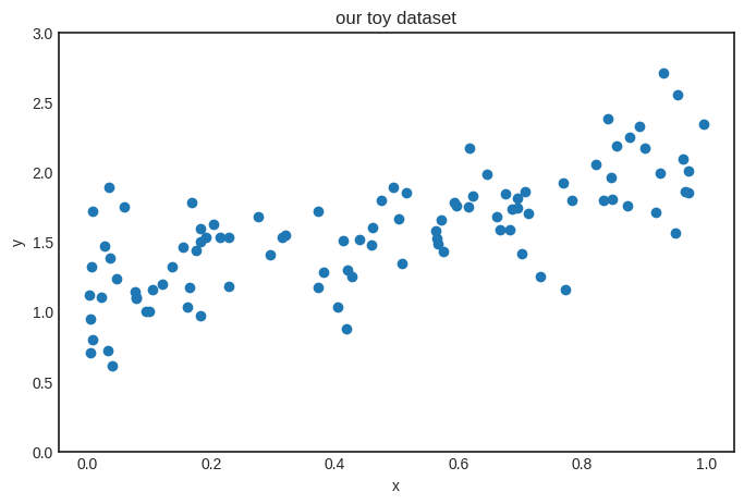
Let’s create the training dataset first. To keep things simple, we’ll use a synthetic dataset that represents the generating process \( 0.8 x + 1.2 + \text{noise} \).

n_train = 100
X_train = np.random.rand(n_train)
Y_train = 0.8*X_train + 1.2 + np.random.normal(scale=0.3, size=n_train)

../_images/e8da928878ef802bb68abc5b9af5aff7e8d6489fbcf5a65dc617b2c2061e7a95.png

Remark 3.4 (The validation and test datasets.)

In real machine learning scenarios, we always aim to have validation and test datasets. The validation dataset is used to gauge the model performance during training, while the test dataset is used for the same purpose after training.

To keep things simple, we won’t use validation and test datasets in this chapter and the next. Don’t worry, we’ll use the proper machine learning methodology later.

For simplicity, our linear model will be represented by a function h(x, a, b) of three arguments: the independent variable \( x \), and the model parameters \( a, b \). (We’ll whip out the vectorized version later for the multivariable linear regression. Brace yourselves.)

def h(x, a, b):
    return a*x + b

Here is the loss function as well.

def L(a, b, X, Y):
    n = len(X)
    return sum([(h(x, a, b) - y)**2 for x, y in zip(X, Y)])/n

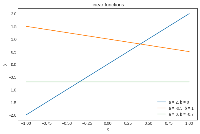
There’s no such thing as too many visualizations. So, here’s the plot of h for various values of \( a \) and \( b \).

../_images/b9f250dda00ee6fc64cca08c3f55a697ff825e1f6edb5b39a2c86ee6db5c313a.png

It’s time to focus on the gradient descent part. First, we implement the gradient \( \nabla L \), given by (3.1) and (3.2).

def grad_L(a, b, X, Y):
    n = len(X)
    da = sum([2*x*(h(x, a, b) - y) for x, y in zip(X, Y)])/n
    db = sum([2*(h(x, a, b) - y) for x, y in zip(X, Y)])/n
    return (da, db)

Everything is lined up to finally train our very first machine learning model. I can almost hear the drums rolling. Here we go.

a_0, b_0 = (0.0, 0.0)    # the initial parameters
lr = 0.01                # the learning rate
n_steps = 150            # the number of optimization steps
ws = [(a_0, b_0)]        # we'll keep our parameters in the list ws

for _ in range(n_steps):
    a_k, b_k = ws[-1]
    da, db = grad_L(a_k, b_k, X_train, Y_train)
    ws.append((a_k - lr*da, b_k - lr*db))

(For simplicity, we don’t check the convergence, just run the iteration for a fixed number of steps which I determined via the scientific method; that is, I played around until things started to work.)

Checking the result. Here are the parameters we have obtained:

f"h(x) = {ws[-1][0]} x + {ws[-1][1]}"

'h(x) = 0.6942667448057251 x + 1.2197490107802043'

The “true” function is \( f(x) + 0.8x + 1.2 \), so the result is quite good. Let’s see the learning algorithm in action: we’ll plot how \( h_k(x) \) is evolving, where \( h_k(x) \) is the solution after the \( k \)-th iteration of gradient descent.

../_images/5ca6cfa7c9060c4e2c13c6930cb847bdd9a97ed03351a22ea5ce7713ea1798a6.png

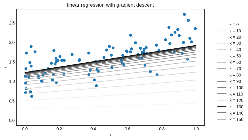
It works! Building something from scratch is not only an incredible feeling, but the best learning experience. (That’s why I insist on implementing everything from scratch.)

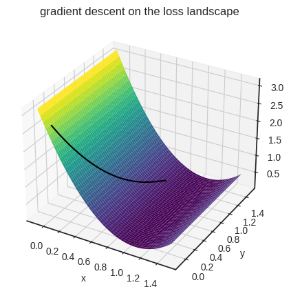
One more thing before we move on. We can also visualize gradient descent on the loss landscape as well. As realistic machine learning scenarios involve loss functions of more than two variables (often millions of them), let’s capitalize on our situation. Check out how gradient descent inches towards an optimum:

../_images/4e628fba27f380d62a7b25099c7b81ba3642a267076b1fe0a0c5802ba0ba6885.png

Now that we understand the fundamentals of linear regression, it’s time to dig deeper.

3.3. Solving the least squares problem#

Using gradient descent for linear regression is like shooting a sparrow with a cannonball. (Especially for a single variable model.) Why? Because the loss function is so simple that we can easily find an analytic solution.

Recall the characterization of the local optima for a function of two variables: if \( \nabla L(\mathbf{w}) = 0 \) and the Hessian determinant \( H_L(\mathbf{w}) \) is positive, then \( \mathbf{w} \) is a local minimum.

Linear regression with the mean-squared error is simple enough to solve \( \nabla L(\mathbb{w}) = 0 \), so let’s give it a shot. This is called the least squares problem, as \( L(\mathbf{w}) \) is composed of squares, and we are supposed to find \( \mathbf{w} \) that makes the least squares. Let’s get to it!

By factoring out the parameters \( a \) and \( b \), we can write (3.1) and (3.2) as

\[\begin{split} \begin{align*} \frac{\partial L}{\partial a} &= \frac{1}{n} \sum_{i=1}^{n} 2 x_i (a x_i + b - y_i) \\ &= \bigg[ \frac{2}{n} \sum_{i=1}^{n} x_i^2 \bigg] a + \bigg[ \frac{2}{n} \sum_{i=1}^{n} x_i \bigg] b - \bigg[ \frac{2}{n} \sum_{i=1}^{n} x_i y_i \bigg] \end{align*} \end{split}\]

and

\[ \begin{align*} \frac{\partial L}{\partial b} &= \bigg[ \frac{2}{n} \sum_{i=1}^{n} x_i \bigg] a + 2 b - \bigg[ \frac{2}{n} \sum_{i=1}^{n} y_i \bigg]. \end{align*} \]

With the powers of linear algebra, we’ll eliminate all this complexity in a heartbeat. It still won’t be pretty, but we’ll polish it to perfection in the later chapters.

First, notice that these sums are awfully familiar: they are dot products in disguise! With the vectorized notation

\[\begin{split} \mathbf{x} = \begin{bmatrix} x_1 \\ \vdots \\ x_n \\ \end{bmatrix} \in \mathbb{R}^n, \quad \mathbf{y} = \begin{bmatrix} y_1 \\ \vdots \\ y_n \\ \end{bmatrix} \mathbb{R}^n, \end{split}\]

we have

\[\begin{split} \begin{align*} \sum_{i=1}^{n} x_i^2 &= \mathbf{x}^T \mathbf{x}, \\ \sum_{i=1}^{n} x_i y_i &= \mathbf{x}^T \mathbf{y}, \\ \sum_{i=1}^{n} x_i &= \mathbf{x}^T \mathbf{1}, \\ \sum_{i=1}^{n} y_i &= \mathbf{y}^T \mathbf{1}, \end{align*} \end{split}\]

where \( \mathbf{1} \) denotes the \( n \)-dimensional vector composed out of ones, and \( \mathbf{x}^T \mathbf{y} \) is the dot product of \( \mathbf{x} \) and \( \mathbf{y} \) in matrix multiplication form. Using this and multiplying the equations (3.1) and (3.2) by \( n/2 \) to get rid of the constants, we obtain the linear system of equations

\[\begin{split} \begin{align*} \frac{\partial L}{\partial a} = (\mathbf{x}^T \mathbf{x}) a + (\mathbf{x}^T \mathbf{1}) b - \mathbf{x}^T \mathbf{y} &= 0, \\ \frac{\partial L}{\partial b} = (\mathbf{x}^T \mathbf{1}) a + n b - \mathbf{y}^T \mathbf{1} &= 0. \end{align*} \end{split}\]

This is much more friendly than the previous version with all those big sums. Solving a \( 2 \times 2 \) linear equation should be standard practice for you by now, so I’ll leave the details up to you, but the solutions are

\[\begin{split} \begin{align*} a &= \frac{n (\mathbf{x}^T \mathbf{y}) - (\mathbf{x}^T \mathbf{1}) (\mathbf{y}^T \mathbf{1})}{n (\mathbf{x}^T \mathbf{x}) - (\mathbf{x}^T \mathbf{1})^2}, \\ b &= \frac{(\mathbf{x}^T \mathbf{x}) (\mathbf{y}^T \mathbf{1}) - (\mathbf{x}^T \mathbf{1}) (\mathbf{x}^T \mathbf{y})}{n (\mathbf{x}^T \mathbf{x}) - (\mathbf{x}^T \mathbf{1})^2}. \end{align*} \end{split}\]

Let’s check if it works!

def solve_least_squares(X, Y):
    n = len(X)
    
    X_dot_Y = np.dot(X, Y)
    X_dot_1 = np.dot(X, np.ones_like(X))
    Y_dot_1 = np.dot(Y, np.ones_like(Y))
    X_dot_X = np.dot(X, X)
    
    a = (n * X_dot_Y - X_dot_1 * Y_dot_1) / (n * X_dot_X - X_dot_1**2)
    b = (X_dot_X * Y_dot_1 - X_dot_1 * X_dot_Y) / (n * X_dot_X - X_dot_1**2)
    
    return a, b

a, b = solve_least_squares(X_train, Y_train)

f"h(x) = {a} x + {b}"

'h(x) = 0.9358010656621849 x + 1.135548284780517'

Here is the result in its full glory.

../_images/35c4d93892391b2687837f538627e7cc9085ce8a9ef8171fc4bf70bbd8ed414f.png

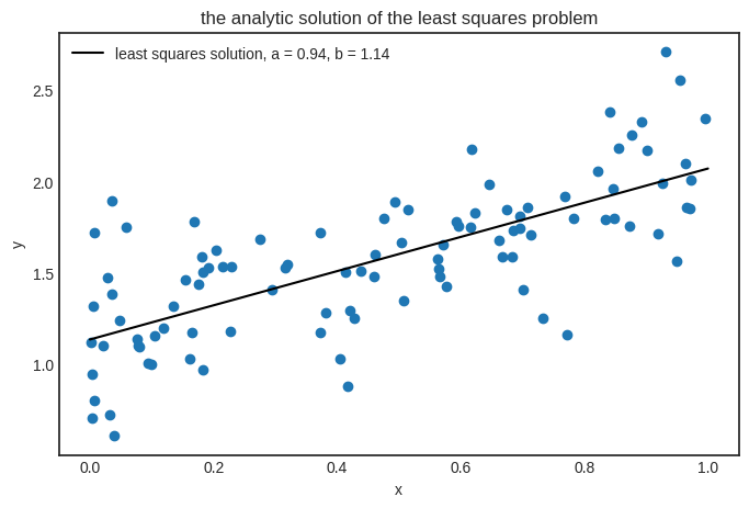
Our least squares solver works perfectly. Then why did we bother with gradient descent, considering that it only provides an approximating solution? Simple: to understand the key ideas using a toy model. In practice, (hopefully) no one will ever fit a linear regression using gradient descent. However, the fitting more complex models is impossible analytically. Linear regression is the exception.

3.4. Linear regression as a Gaussian model#

If you are an intuitive thinker, you probably feel that we never explained why we choose the mean-squared error as the loss function. Sure, it’s mathematically simple and neat, but so is

\[ L^{*}(a, b) = \frac{1}{n} \sum_{i=1}^{n} |h(x_i) - y_i|, \]

where \( | h(x_i) - y_i | \) represents the actual distance between the prediction and the observation, not its transformed version.

One reason is that the absolute value function is not differentiable at zero, but there is another explanation: the linear model and the mean-squared error arises naturally when we assume a statistical mindset.

Take one more look at our toy dataset. Can a function adequately explain our data?

No, because for each given input variable \( x \), our observation clearly has a visible amount of variance.

So, instead of looking to fit a function to the data, we’ll build a probabilistic model. Again, we are looking for simple models, so it’s a safe bet to assume a normal distribution for \( y \).

Translating to the language of probability, let \( X \) and \( Y \) be the two random variables generating our observations. In other words, the inputs \( x_1, \dots, x_n \) are coming from the distribution of \( X \), and the outputs \( y_1, \dots, y_n \) are coming from \( Y \). Mathematically speaking, we are looking to fit a normal distribution on the conditional distribution of \( Y \) given \( X \), that is,

\[ f_{Y \mid X}(y \mid x) = \frac{1}{\sigma \sqrt{2 \pi}} e^{- \frac{(y - \mu(x))^2}{2 \sigma^2}}, \]

where

\( f_{Y \mid X}(y | x) \) is the conditional density function we are looking for,
the right side is the density function of a normal distribution,
\( \mu(x) \) is the expected value (that depends on \( x \)),
and \( \sigma^2 \) is the variance. (Which is assumed to be constant for simplicity.)

Now that our model is ready, it’s time to fit it to the data! In this case, the likelihood function takes the form

\[\begin{split} \begin{align*} \mathrm{LLH}(\mu) &= \prod_{i=1}^{n} f_{Y \mid X}(y_i \mid x_i) \\ &= \prod_{i=1}^{n} \frac{1}{\sigma \sqrt{2 \pi}} e^{- \frac{(y_i - \mu(x_i))^2}{2 \sigma^2}}, \\ \end{align*} \end{split}\]

Maximizing a product is not a simple feat, so we apply a mathematical trick: we take the logarithm to turn the product into a sum. As the logarithm function is increasing, optimizing \( \mathrm{LLH}(\mu) \) is the same as optimizing \( \log \mathrm{LLH}(\mu) \), so the solutions stay the same. Thus, we obtain

\[\begin{split} \begin{align*} \log \mathrm{LLH}(\mu) &= \log \bigg[ \prod_{i=1}^{n} \frac{1}{\sigma \sqrt{2 \pi}} e^{- \frac{(\mu(x_i) - y_i)^2}{2 \sigma^2}} \bigg] \\ &= \sum_{i=1}^{n} \log \bigg[ \frac{1}{\sigma \sqrt{2 \pi}} e^{- \frac{(\mu(x_i) - y_i)^2}{2 \sigma^2}} \bigg] \\ &= \sum_{i=1}^{n} \bigg[ -\frac{(\mu(x_i) - y_i)^2}{2 \sigma^2} + \log \frac{1}{\sigma \sqrt{2 \pi}} \bigg] \\ &= n \log \frac{1}{\sigma \sqrt{2 \pi}} - \frac{1}{2 \sigma^2} \sum_{i=1}^{n} (\mu(x_i) - y_i)^2. \end{align*} \end{split}\]

It’s starting to take shape. As the trendline shows a linear behavior (because it’s how we generated the data ;) ), we can assume that the expected value function is linear; that is, \( \mu(x) = ax + b \).

Thus, the (log-)likelihood function \( \log \mathrm{LLH}(p) = \log \mathrm{LLH}(a, b) \) can be written as

\[ \begin{align*} \log \mathrm{LLH}(a, b) &= n \log \frac{1}{\sigma \sqrt{2 \pi}} - \frac{1}{2 \sigma^2} \sum_{i=1}^{n} (a x_i + b - y_i)^2, \end{align*} \]

where we select the \( a \) and \( b \) that maximizes \( \mathrm{LLH}(a, b) \):

\[ \hat{a}, \hat{b} = \arg \max_{a, b \in \mathbb{R}} \mathrm{LLH}(a, b). \]

Two more adjustments, and we are there. First, as the leading additive constant \( n \log \frac{1}{\sigma \sqrt{2 \pi}} \) does not depend on any of the parameters, we are free to discard it. Same goes for the multiplicative constant \( \frac{1}{2 \sigma^2} \) Second, maximizing \( \log \mathrm{LLH}(a, b) \) is the same as minimizing \( - \log \mathrm{LLH}(a, b) \).

Hence, the maximum likelihood estimation is equivalent with minimizing the loss function

\[\begin{split} \begin{align*} L(a, b) &= - \frac{2 \sigma^2}{n} \bigg[\log \mathrm{LLH}(a, b) - n \frac{1}{\sigma \sqrt{2 \pi}} \bigg] \\ &= \frac{1}{n} \sum_{i=1}^{n} (a x_i + b - y_i)^2, \end{align*} \end{split}\]

which is the good old mean squared error, arising from our probabilistic model. We are back at square one: fitting a Gaussian model with a linear expected value function using maximum likelihood is the same as the plain old linear regression with mean squared error.