6. Entering higher dimensions#
So far, we’ve studied and implemented two machine learning algorithms: linear and logistic regression in a single lonely variable. As always, there’s a hiccup. Real datasets contain way more than one feature. (And they are rarely linear. But we’ll cross that bridge later.)
In this chapter, we’ll take one step towards reality and learn how to handle multiple variables.
First, look at the famous California housing dataset from scikit-learn. The dataset holds of 20640 instances, each consisting of
a vector \( \mathbf{x} \in \mathbb{R}^8 \) of 8 features describing a census block group (such as median income per block, the average number of rooms per household, etc.),
and a target variable \( y \in \mathbb{R} \), containing the median house value for the census block group,
combined in the dataset
Here’s the dataset in its NumPy form.
from sklearn.datasets import fetch_california_housing

housing = fetch_california_housing()
The housing object contains two NumPy arrays: the data and the target. Let’s unpack them and check their shape!
X, Y = housing.data, housing.target
X.shape
(20640, 8)
As the shape (20640, 8) indicates, each row of the matrix X represents a data sample, and each column corresponds to a feature. Here’s a data sample:
X[0]
array([ 8.33, 41.00, 6.98, 1.02, 322.00, 2.56, 37.88, -122.23])
X[0].shape
(8,)
Mathematically speaking, each data sample is a row vector \( \mathbb{R}^{1 \times 8} \), and each feature is a column vector \( \mathbb{R}^{20640 \times 1} \).
Remark 6.1 (The eternal dilemma of row vs column vectors.)
You might have noticed that while data samples come in row vectors, we often use column vectors throughout the study of multivariable functions. Both choices are properly justified: column vectors are convenient for theory, but row vectors are perfect for practice.
To make this extremely (and often redundantly) clear, we’ll indicate this by using the matrix notation \( \mathbb{R}^{1 \times m} \) for row vectors and \( \mathbb{R}^{n \times 1} \) for column vectors.
(However, to lean towards practice, we’ll prefer row vectors from now on.)
On the other hand, the ground truths for the target variable are stored in a massive row vector, represented by the NumPy array Y of shape (20640, ).
Y.shape
(20640,)
Remark 6.2 (Shapes of NumPy arrays.)
In NumPy, the shape of an array is a tuple. In Python, the object (20640) would be interpreted as an integer, hence the comma in Y.shape = (20640,). Thus, for our purposes, shapes like (20640, ) mean that the underlying NumPy array is one-dimensional.
To predict the median house value \( y \in \mathbb{R} \) from the feature vector \( x \in \mathbb{R}^{8} \), we’ll use machine learning. (Surprise.) Mathematically speaking, we are looking for a regression model in the form of a multivariable function \( f: \mathbb{R}^8 \to \mathbb{R} \). Practically speaking, our task is to construct a function that maps an array of shape (8,) into a float.
You all know me well by now: minimizing complexity is one of my guiding principles. So, let’s build a model that is useful and dead simple at the same time. What’s our very first idea when we hear the term “simple”?
Linear regression.
6.1. The generalization of linear regression#
Recall that for a single numerical feature \( x \), the simplest regression model was the linear one; that is, a function of the form \( h(x) = ax + b \) for some \( a, b \in \mathbb{R} \). Intuitively speaking, \( a \) quantified the effect of the feature \( x \) on the target variable \( y \), while \( b \) quantified the bias.
A straightforward generalization is the model
where
\( \mathbf{x} = (x_1, \dots, x_d) \in \mathbb{R}^{1 \times d} \) is a \( d \)-dimensional feature vector,
\( \mathbf{a} = (a_1, \dots, a_d) \in \mathbb{R}^{1 \times d} \) is the regression coefficient vector,
\( b \in \mathbb{R} \) is the bias,
and \( \mathbf{w} = (a_1, \dots, a_d, b) \in \mathbb{R}^{1 \times (d + 1)} \) is the vector of parameters.
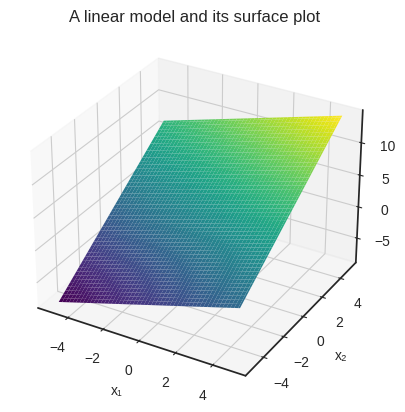
For a given parameter configuration, \( h(\mathbf{x}) \) determines a \( d \)-dimensional plane. It’s simpler to visualize a two-variable example. Here’s a NumPy implementation of a simple linear model with coefficients \( a_1 = 0.8 \), \( a_2 = 1.5 \), and \( b = 3 \).
a = np.array([0.8, 1.5])
b = 3

def an_example_linear_model(x):
    return x @ a.T + b
(The operator @ denotes the matrix multiplication in NumPy.)
The function an_example_linear_model takes a NumPy array of shape (2, ), and returns a float. Nothing special here.
x_in = np.array([-3.8, 0.4])

an_example_linear_model(x_in)
0.56
Here’s the surface plot given by our example \( 0.8 x_1 + 1.5 x_2 + 3 \).
Show code cell source
# Hey! If you are checking this snippet out, keep in mind that it's inefficient
# on purpose.
#
# For instance, one would never call a NumPy function such as
# y[i, j] = an_example_linear_model(np.array([x1s[i, j], x2s[i, j]])),
# which is how I'm doing it below.
#
# We'll talk about vectorized code later in this chapter. For now,
# let's just hack and slash our way towards a simple figure.

import matplotlib.pyplot as plt
from mpl_toolkits.mplot3d import Axes3D
from itertools import product

with plt.style.context('seaborn-v0_8-white'):
    x1s = np.linspace(-5, 5, 100)
    x2s = np.linspace(-5, 5, 100)
    x1s, x2s = np.meshgrid(x1s, x2s)

    i_max, j_max = x1s.shape
    y = np.zeros_like(x1s)
    for i, j in product(range(i_max), range(j_max)):
        y[i, j] = an_example_linear_model(np.array([x1s[i, j], x2s[i, j]]))


    fig = plt.figure()
    ax = fig.add_subplot(111, projection='3d')
    ax.plot_surface(x1s, x2s, y, cmap='viridis')

    ax.set_xlabel('x₁')
    ax.set_ylabel('x₂')
    ax.set_zlabel('y')

    plt.title("A linear model and its surface plot")
    plt.show()
Remark 6.3 (Graph of an affine function’s graph.)
Mathematically speaking, plotting \( h(\mathbf{x}) \) is not enough to prove that the resulting surface is a plane. To do that, we need to show that for all \( \mathbf{x}, \mathbf{y} \in \mathbb{R}^d \) and all \( \lambda \in \mathbb{R} \),
holds. This is because the graph is defined by
and in general, the set
determines the unique line passing through \( \mathbf{u} \) and \( \mathbf{v} \). Thus, (6.1) is translated to the requirement “the line determined by any two points \( h(\mathbf{x}) \) and \( h(\mathbf{y}) \) of the graph also lies on the graph”.
So,
You know the deal by now: we’ll invoke a loss function, fit the model via gradient descent, and test the result. Let’s get to it!
As in the single-variable case, the partial derivatives with respect to the parameters are easily calculated:
Thus, the gradient equals to
Remark 6.4 (More abuse of notations.)
As the number of features increases, so does the number of parameters; as does the number of parameters, so does the notational complexity. Let’s break it down. The hypothesis \( h \) is a function of
the feature vector \( \mathbf{x} \),
and the model parameters \( \mathbf{w} \).
We’ll only need the derivatives with respect to \( \mathbf{w} \) to perform gradient descent. This is indicated in the subscript of the \( \nabla \) symbol:
When the situation is clear, we’ll omit the arguments and write \( \nabla h \) to avoid the explosion of indices and variables.
And if we’re talking about abuse of notation, how about another: let’s write \( (\mathbf{a}, b) \) for concatenating \( \mathbf{a} \) and \( b \):
Again, this is not cheating. If we want to be really mathematician about it, we could show that \( \mathbb{R}^d \times \mathbb{R} \) is the same as \( \mathbb{R}^{d + 1} \). I’ll leave that as an exercise in set theory, but feel free to take my word for it.
Now that we have the gradient, it’s time to fit the model.
6.2. Vectorization#
As our target variable is numerical, the simplest is just to go with the mean squared error once more:
where
\( \mathbf{x}_i = (x_{i, 1}, \dots, x_{i, d}) \in \mathbb{R}^{1 \times d} \) is the \( i \)-th data sample,
\( y_i \) is the ground truth for the sample \( \mathbf{x}_i \),
\( \mathbf{a} = (a_1, \dots, a_d) \in \mathbb{R}^{1 \times d} \) is the regression coefficient,
\( b \in \mathbb{R} \) is the bias,
and \( \mathbf{w} = (\mathbf{a}, b) \in \mathbb{R}^{1 \times (d + 1)} \) is the full parameter vector.
Now comes the gradient. With a simple application of the chain rule and sum rule, we have
and similarly,
Hold on for a second here: when there’s a sum, there’s a dot product! By taking another look at the expression
we can notice that this is the dot product of the vector
and the \( j \)-th column of the data matrix \( X \):
(The vector on the left will only remain anonymous for a short time; we’ll name it soon.)
But hold on for yet another second: when there’s a column vector, there’s a (potential) matrix product! By concatenating a column of ones to the right of \( X \), let’s define
With this, we can write the gradient in the compact form
which is a far cry from the first version with a bunch of sums. This is called vectorization. The form (6.3) is not only simpler to write, but faster to compute.
But hold on for one last time! Speaking of vectorization, let’s revisit our model, defined by
If we formally replace the vector \( \mathbf{x} \) with the matrix \( X \) (whose \( i \)-th row is the vector \( \mathbf{x}_i \)) and define
we have
With this, we can write the gradient (6.3) in the ultimate form
By employing the augmented data matrix \( X_b \) defined by (6.2), we can make this even simpler:
In other words, the definition \( h(X; \mathbf{w}) = X \mathbf{a}^T + \mathbf{b} \) is not just a formal substitution; the expression \( \mathbf{x} \mathbf{a}^T + b \) is correctly evaluated. (With a bit of operator overloading.) In yet another words, we can evaluate the model on a bunch of data samples with a single function call.
This is 1) awesome, and 2) all built-in within NumPy.
Check it out.
a = np.array([1, 2, 3])    # the regression coefficients
b = 4                      # the bias
def h(x):
    return x @ a.T + b
Here’s the result on a vector input…
x = np.array([1, 2, 3])

h(x)
18
…and here’s the result when we plug in a matrix.
X = np.array([[1,  2,  3],
              [4,  5,  6],
              [7,  8,  9],
              [10, 11, 12]])

h(X)
array([18, 36, 54, 72])
h works for both, which is pretty cool.
We can manually check if the expression x @ a.T + b works as intended.
h(X) == np.array([1*1 + 2*2 + 3*3 + 4,
                  4*1 + 5*2 + 6*3 + 4,
                  7*1 + 8*2 + 9*3 + 4,
                  10*1 + 11*2 + 12*3 + 4])
array([ True, True, True, True])
All stars are aligned. Let’s fit the model on some actual data.
6.3. Fitting the model#
It’s time to implement the MultivariateLinearRegressor. We’ll use the interface defined in the previous chapter.
By now, we should be able to do it in a single breath. The gradient descent is the same as in the previous couple of times: we
select a set of initial parameters \( \mathbf{w}_0 \),
then iterate \( \mathbf{w}_{k + 1} = \mathbf{w}_k - \alpha \nabla L(\mathbf{w}_k) \) until convergence,
with some learning rate \( \alpha > 0 \). (We have been using the expression \( \mathbf{w}_{k + 1} = \mathbf{w}_k - \alpha \nabla L(\mathbf{w}_k) \) for quite a while now. It’s time to notice that it is already vectorized!)
We’ll use the regular form \( h(X; \mathbf{w}) = X \mathbf{a}^T + b \), but feel free to implement the augmented matrix version \( h(X; \mathbf{w}) = X_b \mathbf{w}^T \) as well.
class MultivariateLinearRegressor:
    def __init__(self, n_features):
        self.a = np.zeros(n_features)
        self.b = 0

    def __call__(self, X):
        """
        Args:
            X: numpy.ndarray of shape (n_batch, n_features) containing
                the input value.

        Returns:
            Y: numpy.ndarray of shape of shape (n_batch, ) containing
                the model predictions.
        """

        return X @ self.a + self.b

    def _grad_L(self, X, Y):
        """
        Args:
            X: numpy.ndarray of shape (n_batch, in_dim) containing
                the input value.

            Y: numpy.ndarray of shape of shape (n_batch, ) containing
                the corresponding ground truth.

        Returns:
            da: numpy.ndarray of shape (n_features, ) containing
                the gradient with respect to a.

            db: float, containing the gradient with respect to b.
        """

        n = len(X)
        pred_error = self(X) - Y

        da = (2/n) * pred_error @ X
        db = (2/n) * pred_error.sum()
        return da, db

    def fit(self, X, Y, lr=0.01, n_steps=1000):
        """
        Args:
            X: numpy.ndarray of shape (n_batch, in_dim) containing
                the input value.

            Y: numpy.ndarray of shape of shape (n_batch, ) containing
                the corresponding ground truth.

            lr: float describing the learning rate.

            n_steps: integer, describing the number of steps taken by
                the gradient descent.
        """

        for _ in range(n_steps):
            da, db = self._grad_L(X, Y)
            self.a, self.b = self.a - lr*da, self.b - lr*db
Let’s generate some fake training and testing data to test our implementation.
Yes, I know. This book is advertised as “putting practice first” and whatnot, but bear with me for a minute. Generated data makes it easy to study a case when linear regression is guaranteed to work. I promise to try our model on the California housing data soon to see how many ways we can crash and burn.
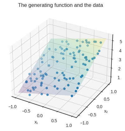
For visualization purposes, we’ll use two features: \( x_1 \) and \( x_2 \). Suppose that our data is generated by the function \( f(\mathbf{x}) = 0.8 x_1 + 1.5 x_2 + 3 \). (This is exactly the function that we used a few sections before.)
a = np.array([0.8, 1.5])
b = 3

def target_function(x):
    return np.dot(x, a) + b
Here’s the (artificial) data.
n_samples = 100
n_features = 2

X = 2*(np.random.rand(n_samples, n_features) - 0.5)
Y = target_function(X) + 0.2*np.random.randn(100)
This is how the data looks, plotted along the target_function’s surface.
Show code cell source
with plt.style.context('seaborn-v0_8-white'):
    x1s = np.linspace(-1, 1, 100)
    x2s = np.linspace(-1, 1, 100)
    x1s, x2s = np.meshgrid(x1s, x2s)

    i_max, j_max = x1s.shape
    y = np.zeros_like(x1s)
    for i, j in product(range(i_max), range(j_max)):
        y[i, j] = target_function(np.array([x1s[i, j], x2s[i, j]]))

    fig = plt.figure()
    ax = fig.add_subplot(111, projection='3d')
    ax.plot_surface(x1s, x2s, y, cmap='viridis', alpha=0.2)

    ax.scatter(X[:, 0], X[:, 1], Y)

    ax.set_xlabel('x₁')
    ax.set_ylabel('x₂')
    ax.set_zlabel('y')
    plt.title("The generating function and the data")
    plt.show()
Now, our trained model is only a .fit call away.
model = MultivariateLinearRegressor(n_features=2)
model.fit(X, Y, lr=0.01, n_steps=1000)

f'The trained model is: h(x) = {model.a[0]:.4g} x₁ + {model.a[1]:.4g}x₂ + {model.b:.4g}'
'The trained model is: h(x) = 0.8658 x₁ + 1.454x₂ + 2.957'
That’s pretty cool! The trained model is quite close to the generating function, so gradient descent works again.
What about the hyped-up California housing dataset? Will our baseline linear model at least work on a real dataset?
Brace for impact.
6.4. An explosion of gradients#
Let’s not waste any time, and jump into the hardcore machine learning. (That is, calling the .fit method.)
X_housing, Y_housing = housing.data, housing.target
n_features = X_housing.shape[1]

model = MultivariateLinearRegressor(n_features)
model.fit(X_housing, Y_housing, lr=0.01, n_steps=1000)
/tmp/ipykernel_23032/1072799047.py:17: RuntimeWarning: overflow encountered in matmul
  return X @ self.a + self.b
/home/tivadar/venvs/mathematics-of-machine-learning/lib/python3.10/site-packages/numpy/core/_methods.py:49: RuntimeWarning: overflow encountered in reduce
  return umr_sum(a, axis, dtype, out, keepdims, initial, where)
/tmp/ipykernel_23032/1072799047.py:59: RuntimeWarning: invalid value encountered in subtract
  self.a, self.b = self.a - lr*da, self.b - lr*db
/tmp/ipykernel_23032/1072799047.py:59: RuntimeWarning: invalid value encountered in scalar subtract
  self.a, self.b = self.a - lr*da, self.b - lr*db
These menacing warnings suggest that something went sideways.
What are the model parameters?
f"The model parameters are a = {model.a} and b = {model.b}."
'The model parameters are a = [ nan nan nan nan nan nan nan nan] and b = nan.'
Damn. nan-s all over the place. This is the very first time we attempted to machine-learn a real dataset, and it all went wrong. Machine learning is hard.
What can be the issue? Those cursed nan-s rear their ugly head when numbers become too large, as in our case. Let’s initialize a brand new model from scratch, and do the gradient descent one step at a time.
model = MultivariateLinearRegressor(n_features)
Here’s the weight gradient of a fresh model.
da, db = model._grad_L(X_housing, Y_housing)
print(f"da = {da})")
print(f"db = {db}")
da = [-19.03 -121.55 -23.33 -4.49 -5832.94 -12.13 -146.70  494.89])
db = -4.137116338178294
We can already see an issue at \( a_5 \): the gradient is orders of magnitude larger there than elsewhere.
Let’s run a gradient descent for a single step and check the gradient. Here’s the weight gradient of a fresh model.
model.fit(X_housing, Y_housing, lr=0.01, n_steps=1)

da, db = model._grad_L(X_housing, Y_housing)
print(f"da = {da}")
print(f"db = {db}")
da = [ 650134.30  4309357.94  886578.58  179715.84  388576418.37  610690.14
  5943142.34 -20019855.00]
db = 167652.8761973431
Things go crazy after just one step!
What can we do? The simplest idea is to lower the learning rate. After all, the learning rate is the multiplier of the gradient in the weight update equation. Let’s try \( 0.000001 \), or 1e-6 in scientific notation!
model = MultivariateLinearRegressor(n_features)
model.fit(X_housing, Y_housing, lr=1e-6, n_steps=1000)

f"The model parameters are a = {model.a} and b = {model.b}."
/tmp/ipykernel_23032/1072799047.py:59: RuntimeWarning: invalid value encountered in subtract
  self.a, self.b = self.a - lr*da, self.b - lr*db
/tmp/ipykernel_23032/1072799047.py:59: RuntimeWarning: invalid value encountered in scalar subtract
  self.a, self.b = self.a - lr*da, self.b - lr*db
'The model parameters are a = [ nan nan nan nan nan nan nan nan] and b = nan.'
Still nan. Let’s shift the decimal to the right and see what happens if the learning rate is set to 1e-7!
model = MultivariateLinearRegressor(n_features)
model.fit(X_housing, Y_housing, lr=1e-7, n_steps=1000)

print(f"The model parameters are a = {model.a}")
print(f"and b = {model.b}.")
The model parameters are a = [ 0.00  0.00  0.00  0.00  0.00  0.00  0.00 -0.01]
and b = 9.08681864688336e-05.
Just one small step down in the learning rate, and instead of exploding, gradient descent got stuck at the start. Sure, we can try to find a value between 1e-6 and 1e-7, perhaps let the gradient descent run longer, but those won’t solve our problem.
Let me show you the crux of the issue. Here are the first five rows of the data matrix.
X_housing[:5]
array([[ 8.33,  41.00,  6.98,  1.02,  322.00,  2.56,  37.88, -122.23],
       [ 8.30,  21.00,  6.24,  0.97,  2401.00,  2.11,  37.86, -122.22],
       [ 7.26,  52.00,  8.29,  1.07,  496.00,  2.80,  37.85, -122.24],
       [ 5.64,  52.00,  5.82,  1.07,  558.00,  2.55,  37.85, -122.25],
       [ 3.85,  52.00,  6.28,  1.08,  565.00,  2.18,  37.85, -122.25]])
The real problem is that the features are on a completely different scale. Check out the distribution of each feature, visualized on a barplot.
Show code cell source
import seaborn as sns
import pandas as pd

with plt.style.context('seaborn-v0_8-white'):
    df = pd.DataFrame(X_housing, columns=[f'Feature {i+1}' for i in range(X_housing.shape[1])])
    df_melted = df.melt(var_name='Features', value_name='Values')

    plt.figure(figsize=(10, 6))
    sns.violinplot(x='Features', y='Values', data=df_melted)
    plt.title('Distribution of the features of the housing dataset')
    plt.show()
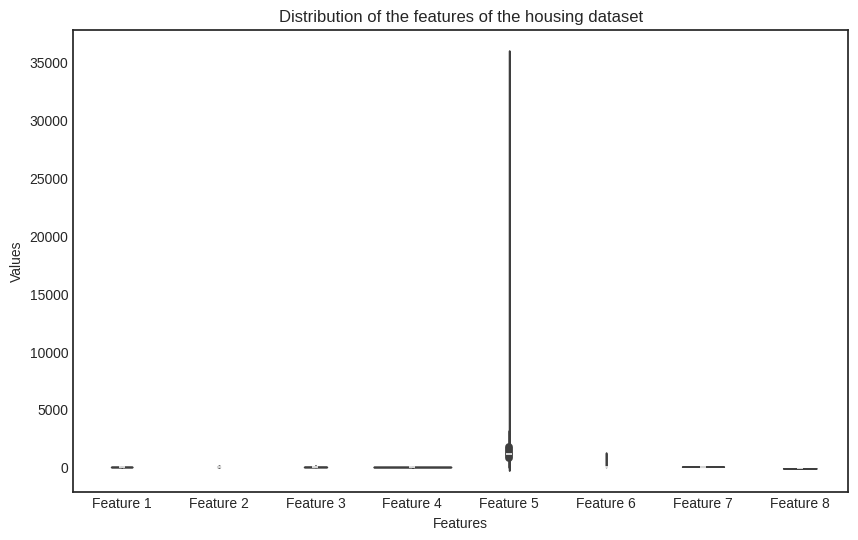
Uh-oh. The issue is glaring. What can we do?
For one, we can transform the features to roughly the same scale and then use the transformed dataset to train a model. Let’s do that!
6.4.1. Scaling the data - in theory#
Mathematically speaking, we aim to find a scaler function \( S: \mathbb{R}^d \to \mathbb{R}^d \) to transform the dataset and then train the multivariate linear regression model on the scaled dataset
where \( \mathcal{D} = \{ (\mathbf{x}_i, y_i): i = 1, 2, \dots, n \}) \) is the original dataset.
How can we conjure up such a function? As we don’t want to mix the features, the simplest is to look for a function in the form
that is, an affine transformation in each feature. Geometrically, the component \( (x_i - \mu_i)/\sigma_i \)
shifts the mean of the feature \( x_i \) via \( x_i - \mu_i \),
then scales the variance of the shifted data by \( \frac{x_i - \mu_i}{\sigma_i} \).
In vectorized terms, \( S(\mathbf{x}) \) can be written in the form
where \( \sigma \in \mathbb{R}^{d \times d} \) is the diagonal matrix
and \( \mu \in \mathbb{R}^{1 \times d} \) is the column vector \( \mu = [\mu_1, \dots, \mu_d]^T \). (Recall that to invert a diagonal matrix, one simply takes the reciprocal of the diagonal elements.)
How do we find the parameters \( \sigma_i \) and \( \mu_i \)? The Greek notation is very suggestive. There are multiple solutions, but the most straightforward is to use the sample means
and sample standard deviations
obtaining the explicit form
If we apply \( S \) to every data sample — that is, every row of the data matrix \( X \) — and stack them on top of each other, we obtain the scaled feature matrix
as stacking row vectors yields a matrix.
Why do we prefer this particular choice? Because the scaled features are standardized, that is, their sample mean is zero and their sample variance is one! I’ll show you why, but first, be brave and pick up a piece of paper to verify this yourself.
It’s a simple calculation: first, the sample mean of the \( j \)-th column is
Second, the sample variance is
Thus, the features are centered at zero and are on the same scale.
Quoting Detective Columbo, just one more thing. All in all, \( S(\mathbf{x}) \) is an affine function. Must we apply it to all data samples individually? No! With a bit of an abuse of notation, if we write
the scaled feature matrix can be written in the form
This is great, especially when it comes to cold, hard practice, which we are just about to see.
6.4.2. Scaling the data - in practice#
Implementation time. First, we’ll do the NumPy version of the scaling function; then we’ll come up with an interface to fit the entire thing into our machine-learning pipeline.
As NumPy allows us to write properly vectorized code without having to worry about manually overloading the operations (such as blowing up the vector of feature means into a matrix), we’ll store the \( 2 \cdot d \) parameters of the function \( S(\mathbf{x}) = ( \mathbf{x} - \widehat{\mu} )^T \widehat{\sigma}^{-1} \) in two vectors.
Here we go.
def scaler(x, mu, sigma):
    return (x - mu)/sigma
It’s that simple. Thanks to NumPy, scaler works for multiple input types! Let’s put it to the test.
X = np.array([[0, 1],
              [2, 3],
              [4, 5],
              [6, 7],
              [8, 9]])
mu = np.array([1, 5])
sigma = np.array([-1, 10])

print(f"X.shape = {X.shape}")
print(f"mu.shape = {mu.shape}")
print(f"sigma.shape = {sigma.shape}")
X.shape = (5, 2)
mu.shape = (2,)
sigma.shape = (2,)
In theory, subtraction between a matrix of dimensions (5, 2) and a vector of (2, ) dimension shouldn’t work; neither does multiplication. However, the broadcasting rules of NumPy allow us to perform the operations we want. In the expression X - mu, NumPy horizontally stacks the vector mu until its shape matches X, then performs the elementwise subtraction.
See for yourself:
X - mu
array([[-1, -4],
       [ 1, -2],
       [ 3,  0],
       [ 5,  2],
       [ 7,  4]])
Similarly, (X - mu)/sigma horizontally stacks sigma until the shapes match, then does the elementwise multiplication with (X - mu)/sigma.
(X - mu)/sigma
array([[ 1.00, -0.40],
       [-1.00, -0.20],
       [-3.00,  0.00],
       [-5.00,  0.20],
       [-7.00,  0.40]])
Thus, scaler performs just what we need. It’s time to integrate data scaling into our machine learning pipeline!
6.4.3. Scaling the data - in our pipeline#
In a machine learning scenario, we can’t just add a scaler function; we need additional functionality. We want to
adapt the scaling parameter to our data,
apply the same scaling during both training and prediction,
and compose it with
MultivariateLinearRegressorin a single pipeline.
Here’s our object-oriented implementation, following the same lines as our previous models.
class DataScaler:
    def __call__(self, X):
        return self.encode(X)

    def fit(self, X):
        """
        Args:
            X: numpy.ndarray of shape (n_batch, in_dim) containing
                the training data.
        """

        self.X_std = X.std(axis=0)
        self.X_mean = X.mean(axis=0)

    def encode(self, X):
        return (X - self.X_mean)/self.X_std

    def decode(self, X):
        return X*self.X_std + self.X_mean
With a DataScaler instance, we can “learn” the scaling parameters and apply them to any sample with the encode method. We can even decode any feature-scaled sample with the decode method.
scaler = DataScaler()
scaler.fit(X_housing)

X_housing_scaled = scaler(X_housing)
Check out the newly scaled features.
Show code cell source
with plt.style.context('seaborn-v0_8-white'):
    df = pd.DataFrame(X_housing_scaled, columns=[f'Scaled\nfeature {i+1}' for i in range(X_housing.shape[1])])
    df_melted = df.melt(var_name='Scaled features', value_name='Values')

    plt.figure(figsize=(10, 6))
    sns.violinplot(x='Scaled features', y='Values', data=df_melted)
    plt.title('Distribution of the features of the housing dataset')
    plt.show()
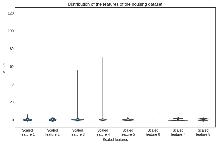
Although there are still differences in the order of magnitude (check out the scaled feature no. 6), the situation is much better.
Remember that scaling is a one-way street: if we train a model on scaled data, we must perform the very same scaling during inference! So, let’s put DataScaler together with MultivariateLinearRegressor into a makeshift pipeline.
class Pipeline:
    def __init__(self, n_features):
        self.scaler = DataScaler()
        self.model = MultivariateLinearRegressor(n_features)

    def __call__(self, X):
        X_scaled = self.scaler(X)
        Y = self.model(X_scaled)
        return Y

    def fit(self, X, Y, lr=0.01, n_steps=1000):
        self.scaler.fit(X)
        X_scaled = self.scaler(X)
        self.model.fit(X_scaled, Y, lr, n_steps)
pipeline = Pipeline(n_features)
pipeline.fit(X_housing, Y_housing, lr=0.01, n_steps=1000)
No warnings so far. Let’s check the model parameters one more time.
f"The model parameters are a = {pipeline.model.a} and b = {pipeline.model.b}."
'The model parameters are a = [ 0.84 0.15 -0.23 0.26 0.01 -0.04 -0.68 -0.65] and b = 2.0685581656078242.'
Yay! It works, and we have a valid model.
Is it any good? We’ll find out in the next chapter, when we finally discuss model evaluation methods.