The backward pass (in practice)

11. The backward pass (in practice)#

In the previous chapter, we have learned about backpropagation; now, it’s time to implement it. We’ll continue where we left off with our Scalar class. To make it suitable for backpropagation, we need to make some enhancements:

have Scalars track the backward derivatives,
and store the local derivatives along the incoming edges.

The first one is already there via the Scalar.backwards_grad attribute. As its value is calculated, we do not allow setting it upon initialization, but set it to zero instead. (I have named it backwards_grad instead of backwards_derivative to match the interface of our future Tensor class. I know, I am a bit of an overthinker.)

Now, onto the meaty parts!

11.1. Tracking the local derivatives#

In the current version of Scalars, we only track the previous nodes. Recall how it behaves in action. (Here’s the current implementation as well, if you want to recall. You have to open it manually although; I don’t want to clutter the text with it.)

a = Scalar(3)
b = Scalar(4)
c = a - b

c.prevs

[Scalar(3), Scalar(-4)]

To carry out the backpropagation, we have to know the local derivatives along the edges. There are many possible solutions; we’ll add a simple Edge data structure to populate Scalar.prevs with.

from collections import namedtuple

Edge = namedtuple("Edge", ["prev", "local_grad"])

Edge is a namedtuple, which is just a fancy way of implementing a simple class with the attributes prev and local_grad.

a = Scalar(1)
e = Edge(prev=a, local_grad=42)

e.prev

Scalar(1)

e.local_grad

From now on, the Scalar.prevs attribute will be populated with Edge objects. So, we have to modify the operations accordingly. For instance, let’s take a look at addition function \( +(x_1, x_2) = x_1 + x_2 \). With this slightly unusual notation, the local derivatives are

\[ \frac{\partial +}{\partial x_1} = \frac{\partial +}{\partial x_2} = 1. \]

Thus, the Scalar defined by x1 + x2 will have two Edge objects in its prevs attribute: Edge(x1, 1) and Edge(x2, 1). This is how it’s done.

class Scalar(Scalar):
    # ...

    def __add__(self, other):
        if not isinstance(other, Scalar):
            other = Scalar(other)

        return Scalar(
            value=self.value + other.value,
            prevs=[Edge(self, 1), Edge(other, 1)],
        )

    # ...    

Can you figure out the rest of the operations? Give this exercise a try. Here, let me provide a template; the rest is up to you. Implement __mul__, __truediv__, and __pow__ so that it keeps track of all the incoming edges during the operations.

(You can use Python’s math.log function from the built-in math module.)

import math


class Scalar(Scalar):
    def __add__(self, other):
        if not isinstance(other, Scalar):
            other = Scalar(other)

        return Scalar(
            value=self.value + other.value,
            prevs=[Edge(self, 1), Edge(other, 1)],
        )

    # implement these methods along the lines of __add__:    
    def __mul__(self, other):
        pass

    def __truediv__(self, other):
        pass

    def __pow__(self, exponent):
        pass

    # auxiliary operations
    def __radd__(self, other):
        return self + other

    def __sub__(self, other):
        return self + (-other)

    def __rsub__(self, other):
        return other + (-self)

    def __rmul__(self, other):
        return self * other

    def __neg__(self):
        return (-1) * self

    def __rtruediv__(self, other):
        if not isinstance(other, Scalar):
            other = Scalar(other)

        return other / self

Ready? Compare your solution to mlfz’s implementation:

Let’s test it out.

a = Scalar(0.5) + Scalar(1.5)
b = a ** Scalar(3)
c = b / Scalar(2)

print(f"a = {a}, b = {b}, c = {c}")

a = Scalar(2.0), b = Scalar(8.0), c = Scalar(4.0)

c.prevs

[Edge(prev=Scalar(8.0), local_grad=0.5), Edge(prev=Scalar(2), local_grad=-2.0)]

b.prevs

[Edge(prev=Scalar(2.0), local_grad=12.0),
 Edge(prev=Scalar(3), local_grad=5.545177444479562)]

a.prevs

[Edge(prev=Scalar(0.5), local_grad=1), Edge(prev=Scalar(1.5), local_grad=1)]

Awesome! Now, we are ready to take the first step backwards, and propagate the derivatives back to the previous nodes.

11.2. A step backwards#

Recall our pseudo-algorithm for backpropagation:

for v in nodes:
    # the backward step for v
    for prev, local_grad in v.prevs:
        prev.backwards_grad += v.backwards_grad * local_grad

In English:

the outer loop iterates through all the nodes,
while the inner loop represents a single backward step.

Although the order of nodes to visit is unclear, notice that the inner part is not pseudocode anymore!

class Scalar(Scalar):
    # ...
    
    def _backward_step(self):
        for prev, local_grad in self.prevs:
            prev.backwards_grad += local_grad * self.backwards_grad

    # ...

(We prefix the backward step with an underscore to indicate that it is not supposed to be called from the outside.)

Let’s test it out.

a = Scalar(2)
b = Scalar(3)
c = a * b

# setting the backwards grad
# (this'll be done automatically)

c.backwards_grad = 4
c._backward_step()

a.backwards_grad should be 12, while b.backwards_grad should be 8.

a.backwards_grad == 12

True

b.backwards_grad == 8

True

Now, we are ready to connect the dots by doing the entire backward pass, involving all nodes. But how?

11.3. All the steps backwards#

Let’s take a look at where we stand. There is only one pseudo-part in our pseudo-algorithm:

for v in nodes:
    v._backward_step()

What is the nodes iterable? Let’s figure this out.

11.3.1. The reversed topological ordering#

When implementing the backward step, we have made a hidden assumption: when we call v._backward_step(), we assume that the backwards derivative v.backwards_grad is already computed. As v receives gradient updates from all of its children, we have to make sure that they are visited previously. So, the order of nodes matters.

This is satisfied by the so-called reversed topological ordering. Here’s the mathematical definition.

Definition 11.1 (Topological ordering of directed graphs.)

Let \( G = (V, E) \) a directed graph.

(i) We say that \( V = {v_1, v_2, \dots, v_n} \) is in topological order, if for any \( (v_i, v_j) \in E \), \( i < j \) holds.
(ii) We say that \( V = {v_1, v_2, \dots, v_n} \) is in reverse topological order, if for any \( (v_i, v_j) \in E \), \( j < i \) holds.

Let’s see an example. For the sake of simplicity, we’ll go with the computational graph given by the expression sigmoid(a * x + b) + a. With the intermediary variables

c = a * x,
d = a * x + b (which is d = c + b),
e = sigmoid(a * x + b) (which is e = sigmoid(d)),
and y = sigmoid(a * x + b) + a (which is y = e + a),

we have the following graph.

../_images/152229b299fad68adb31b511a2316197e1e7b6b228b6fc5291a55f1306efb28d.svg

To compute \( \frac{dy}{da} \), we employ the chain rule, telling us that

\[ \frac{dy}{da} = \frac{dy}{dc} \frac{\partial c}{\partial a} + \frac{dy}{dy}\frac{\partial y}{\partial a}. \]

In other words, \( \frac{dy}{dc} \) must be computed before \( \frac{dy}{da} \). Here, a correct reverse topological ordering would be [y, e, d, b, c, a, x].

How to find the reversed topological ordering of our computational graphs? You know, the ones that are defined via the Scalar objects. Here’s a possible implementation.

class Scalar(Scalar):   
    # ...

    def _get_graph(self):
        ordered_scalars = []
        visited_scalars = set()

        def traverse_graph(x):
            if x not in visited_scalars:
                visited_scalars.add(x)

                for prev, _ in x.prevs:
                    traverse_graph(prev)

                ordered_scalars.append(x)

        traverse_graph(self)

        return ordered_scalars
    
    # ...

In English, the Scalar._get_graph method recursively travels the computational graph. Check out the traverse_graph function that is called for each node: it appends the input node to the ordered_scalars list only when all of its parents are traversed. This way, the topological order is preserved; thus, ordered_scalars contains a topologically ordered list of all Scalar nodes.

So, here’s our (not so) pseudo-backpropagation:

for v in reversed(y._get_graph()):
    v._backward_step()

(Where y is the terminal node of our graph, and reversed is a built-in tool of Python that reverses iterators.)

Let’s not waste any more time and implement this right away!

11.3.2. Completing the backward pass#

We are almost done; in fact, we have all the pieces ready. Let’s combine the Scalar._backward_step and Scalar._get_graph methods together in the Scalar.backward.

(One small modification to _get_graph: we add an option to zero out the backward derivatives. This is needed to make sure our computations don’t overflow into the subsequent passes.)

class Scalar(Scalar):
    # ...

    def _backward_step(self):
        for prev, local_grad in self.prevs:
            prev.backwards_grad += local_grad * self.backwards_grad

    def _get_graph(self, zero_grad=False):
        ordered_scalars = []
        visited_scalars = set()

        def traverse_graph(x):
            if x not in visited_scalars:
                visited_scalars.add(x)

                if zero_grad:
                    x.backwards_grad = 0

                for prev, _ in x.prevs:
                    traverse_graph(prev)

                ordered_scalars.append(x)

        traverse_graph(self)

        return ordered_scalars

    def backward(self):
        ordered_scalars = self._get_graph(zero_grad=True)

        self.backwards_grad = 1

        for scalar in reversed(ordered_scalars):
            scalar._backward_step()

    # ...

The Scalar.backwards method does as what we stated in our pseudoalgorithm, with setting the backwards gradient to one. (Recall that the default value of Scalar.backwards_grad is 0, but the global derivative of a node with respect to itself is 1.)

11.4. Backpropagation in action#

We’ve finally implemented backpropagation, the soul of computational graphs. It’s time to see it in practice.

Let’s stick with the simplest possible example: a linear model, for instance, \( y = 2 x - 1 \). It’s easy to see that \( \frac{dy}{dx} = 2 \), so let’s check if that’s indeed the case.

a = Scalar(2)
b = Scalar(-1)


def linear(x: Scalar):
    return a*x + b

x = Scalar(42)
y = linear(x)

y.backward()

Scalar.backward runs without error, so we’re halfway there. What are the results?

y.backwards_grad

x.backwards_grad

Just as we expected! Let’s check if it works for other inputs.

import numpy as np


xs = [Scalar(x) for x  in np.linspace(-10, 10, 1000)]
dydxs = [x.backwards_grad for x in xs if linear(x).backward() or 1]

np.all([dydx == 2 for dydx in dydxs])

np.True_

Awesome! Let’s move on to a harder example.

11.4.1. Verifying backpropagation#

Now that we have all our ducks in a row, let’s use a more complex computational graph to check if our implementation indeed works. Moving on from linear models, we’ll use the previously seen sigmoid(a * x + b) + a.

The Scalar interface have changed quite a lot since the last time we implemented functions, so let’s revisit the sigmoid. Here’s the vanilla version.

def _sigmoid(x):
    return 1/(1 + np.exp(-x))

def _sigmoid_prime(x):
    return _sigmoid(x) * (1 - _sigmoid(x))

Let’s scalarize this.

def sigmoid(x: Scalar) -> Scalar:
    return Scalar(
        value=_sigmoid(x.value),
        prevs=[Edge(x, _sigmoid_prime(x.value))]
    )

Now, we are ready for sigmoid(a * x + b) + a.

a = Scalar(2)
b = Scalar(-1)

def f(x):
    return sigmoid(a * x + b) + a

You can verify by hand that the derivative of \( f \) is

\[\begin{split} \begin{align*} \frac{df}{dx} &= a \sigma^\prime(a x + b) \\ &= a \sigma(ax + b) \big(1 + \sigma(ax + b) \big), \end{align*} \end{split}\]

so let’s plot this side-by-side with the result of backpropagation.

def f_prime(x):
    return a.value * _sigmoid_prime(a.value * x + b.value)

xs_np = np.linspace(-5, 5, 1000)
xs = [Scalar(x) for x  in xs_np]

dydxs = [x.backwards_grad for x in xs if f(x).backward() or 1]
dydxs_np = f_prime(xs_np)

../_images/3c8519e6e6bfad85906692aafbde2dd5c934fe49b0f34527f5c58f1c1115c5b6.png

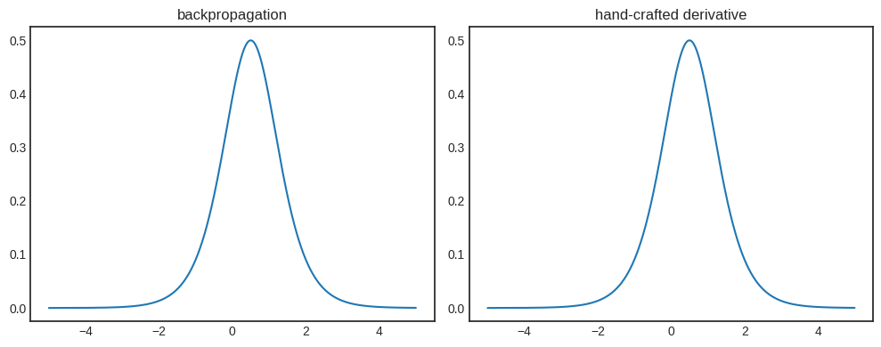
We happy, Vincent? We happy.

11.4.2. Verification via finite differences#

I hate to break it to you, but a side-by-side plot is not enough to convince me of correctness. Sure, it’s a great indication that we are on the right track, but it’s far from adequate.

We need actual tests to see if the backpropagation is implemented correctly. One method is to compute the derivative via finite differences: if \( f \) is a differentiable function and \( h > 0 \) is a number small enough, then

\[ f^\prime(x) \approx \frac{f(x + h) - f(x - h)}{2h}. \]

This way, we can numerically estimate the derivative, and check if the results of backpropagation are close or not. We’ll use the example from the previous section.

a = Scalar(2)
b = Scalar(-1)

def f(x):
    return sigmoid(a * x + b) + a

Computing the finite differences is quite straightforward.

def finite_diff(f, x, h=1e-8):
    result = (f(x + h) - f(x - h))/(2*h)
    return result

xs = [Scalar(x) for x in np.linspace(-10, 10, 1000)]
diffs_fd = [finite_diff(f, x, h=1e-4).value for x in xs]

Here are the results of backpropagation as well.

diffs_bw = [x.backwards_grad for x in xs if f(x).backward() or 1]

(To compute the derivatives with backpropagation, I have used the f(x).backward() or 1 hack to perform the backward pass before adding x.backwards_grad to the list. The expression f(x).backward() or 1 is always true, but Python always evaluates f(x).backward() as well. This trick is good to have in your toolbox.)

Do the results match?

np.allclose(diffs_fd, diffs_bw)

True

Yes! We can relax now, our work is correct.

At this point, you are wondering why are we not using finite differences instead of backpropagation. I give you one: notice that the expression

\[ \frac{f(x + h) - f(x - h)}{2h} \]

requires two forward passes, \( f(x + h) \) and \( f(x - h)\). For \( m \) parameters, we have to compute the finite differences \( m \) times. That’s a lot of forward passes. On the other hand, backpropagation requires a single backward pass.

There’s only one thing missing from Scalar. We’ve gone quite a long way, but we still haven’t trained any model. Let’s see how it’s done in the next chapter!