13. Vectorized computational graphs#
Although Scalar provides a complete implementation for computational graphs, they are terribly hard to work with, not to mention their performance issues. As we’ve seen it earlier, training a simple neural net with a hidden layer of eight Scalar neurons takes a lot of time, and defining it without matrix multiplications is a pain.
Fortunately, we don’t have to be so granular when defining computational graphs. Via the magic of linear algebra, we can seriously cut down the number of nodes and edges in our graphs, resulting in a blazing increase in speed and notational simplicity.
To give you an example, consider the dot product operation, defined by
This is a computational graph that contains \(4n - 1 \) nodes and \(4n - 2 \) edges. Here it is for three-dimensional vectors.

Consider doing a backward pass in this graph: you have to traverse every node, every edge, and execute functions there. It’s even worse for matrix multiplications, and the computational complexity piles up fast. For a basic one-layer network like \( \sigma(\mathrm{ReLU}(xA)B) \), we already have a ton of components. If the inputs are images, we are in the tens of thousands. That’s not going to work out in the long run.
What if we replace scalars with vectors and matrices in our computational graphs?
This is how the dot product would look like:

Structurally, this is identical to the one of matrix multiplication:

This is what the Tensor class implements in mlfz. Let’s see what tensors are!
13.1. How to work with Tensor#
Similarly to Scalar, the Tensor class is a node in a computational graph. This time, instead of a scalar value, they represent NumPy arrays.
import numpy as np
from mlfz.nn.tensor import Tensor


x = Tensor.ones(3, 4)
y = Tensor.zeros_like(x)
x + y
Tensor([[1., 1., 1., 1.],
       [1., 1., 1., 1.],
       [1., 1., 1., 1.]])
A Tensor can be initialized in multiple ways; the principal one is via a NumPy array.
Tensor(np.array([[1, 2], [3, 4]]))
Tensor([[1, 2],
       [3, 4]])
Tensor.from_random(2, 4)
Tensor([[0.44753265, 0.63713811, 0.30274584, 0.62520603],
       [0.18116229, 0.80732081, 0.85423734, 0.12697534]])
Tensor.zeros(5, 2)
Tensor([[0., 0.],
       [0., 0.],
       [0., 0.],
       [0., 0.],
       [0., 0.]])
x = Tensor.zeros(3, 4)
Tensor.ones_like(x)
Tensor([[1., 1., 1., 1.],
       [1., 1., 1., 1.],
       [1., 1., 1., 1.]])
Just like a Scalar, Tensor instances hold three important attributes as well:
a tensor value,
the backwards gradient,
and the list of incoming edges.
x = Tensor.ones(3, 4)
y = Tensor.ones(3, 4)
z = x * y
z.backwards_grad # this is a NumPy array
array([[0., 0., 0., 0.],
       [0., 0., 0., 0.],
       [0., 0., 0., 0.]])
z.prevs # and this is a list of Edges
[Edge(prev=Tensor([[1., 1., 1., 1.],
        [1., 1., 1., 1.],
        [1., 1., 1., 1.]]), local_grad=array([[1., 1., 1., 1.],
        [1., 1., 1., 1.],
        [1., 1., 1., 1.]]), backward_fn=<function _pointwise at 0x73626ad7a0c0>),
 Edge(prev=Tensor([[1., 1., 1., 1.],
        [1., 1., 1., 1.],
        [1., 1., 1., 1.]]), local_grad=array([[1., 1., 1., 1.],
        [1., 1., 1., 1.],
        [1., 1., 1., 1.]]), backward_fn=<function _pointwise at 0x73626ad7a0c0>)]
We’ll talk about the Edge object later, but if you are observant, you may have noticed that compared to the Scalar version, we have an additional backward_fn attribute. This is the price we pay for vectorization.
First, let’s see what Tensors can do.
13.2. Tensors and operations#
Tensors support quite a few operations:
pointwise addition
+,pointwise subtraction
-,pointwise multiplication
*,pointwise division
/,pointwise exponentiation
**,matrix multiplication
@,and matrix transposition
T.
Thanks to the broadcasting magic of NumPy, the other operand need not be a Tensor, it can be a vanilla Python number. (We’ll open a whole other can of worms with broadcasting, but we’ll cross that bridge later.)
x = Tensor.ones(3, 4)
2 + x
Tensor([[3., 3., 3., 3.],
       [3., 3., 3., 3.],
       [3., 3., 3., 3.]])
Just like Scalars, we can apply functions to Tensors.
from mlfz.nn.tensor.functional import exp

x = Tensor(value=np.array([[1, 2], [3, 4]]))
exp(x)
Tensor([[ 2.71828183,  7.3890561 ],
       [20.08553692, 54.59815003]])
As a Tensor is essentially a wrapper over NumPy arrays, it has its own sum and mean methods, working identically to the original versions.
x = Tensor.ones(3, 4)
x.sum()
Tensor(12.)
x.sum(axis=0)
Tensor([3., 3., 3., 3.])
x.sum(axis=1)
Tensor([4., 4., 4.])
y = Tensor(np.array([[1, 2], [3, 4]]))
y.mean()
Tensor(2.5)
y.mean(axis=0)
Tensor([2., 3.])
13.3. Computational graphs with Tensors#
Just like most features, the graph-building is the same as well: it is dynamically built upon applying functions and operations.
from mlfz.nn.tensor.functional import sigmoid, tanh

x = Tensor.from_random(1, 3)
A = Tensor.from_random(3, 5)
B = Tensor.from_random(5, 1)

y = sigmoid(tanh(x @ A) @ B)
y
Tensor([[0.8497897]])
y.shape
(1, 1)
Again, the y.backward method calculates the gradient of y with respect to all nodes in the graph. As our nodes are tensors, the backwards gradient will be a tensor as well, with the shape matching the node’s shape.
y.backward()
x.backwards_grad
array([[0.02344552, 0.09243718, 0.05054987]])
A.backwards_grad
array([[0.00370821, 0.00396276, 0.02496024, 0.06280291, 0.0114475 ],
       [0.00496636, 0.00530728, 0.03342898, 0.08411127, 0.01533152],
       [0.00090712, 0.00096939, 0.00610589, 0.01536313, 0.00280034]])
B.backwards_grad
array([[0.11902051],
       [0.1178138 ],
       [0.10175171],
       [0.06213271],
       [0.08277062]])
In essence, tensors allow us to vectorize computational graphs, increasing the speed and simplicity like you wouldn’t believe. Let’s proceed to build one!
13.4. Building a vectorized neural network with tensors#
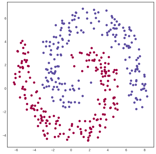
To demonstrate the power of Tensor, we’ll need a dataset to test out our neural network. We’ll use our good old friend, the spiral dataset. (Once again, the dataset generating code is irrelevant, so don’t hung up on it.)
Show code cell source
import numpy as np
from mlfz.nn import Tensor


def generate_spiral_dataset(n_points, noise=0.5, twist=380):
    random_points = np.sqrt(np.random.rand(n_points)) * twist * 2 * np.pi / 360

    class_1 = np.column_stack((-np.cos(random_points) * random_points + np.random.rand(n_points) * noise,
                               np.sin(random_points) * random_points + np.random.rand(n_points) * noise))
    class_2 = np.column_stack((np.cos(random_points) * random_points + np.random.rand(n_points) * noise,
                               -np.sin(random_points) * random_points + np.random.rand(n_points) * noise))

    xs = np.vstack((class_1, class_2))
    ys = np.hstack((np.zeros(n_points), np.ones(n_points))).reshape(-1, 1)

    return Tensor(xs), Tensor(ys)
xs, ys = generate_spiral_dataset(200, noise=2)
Show code cell source
import matplotlib.pyplot as plt


with plt.style.context("seaborn-v0_8-white"):
    plt.figure(figsize=(8, 8))
    plt.scatter([x[0] for x in xs], [x[1] for x in xs], c=ys, cmap=plt.cm.Spectral)
    plt.show()
To define a network, we’ll use the Model class from mlfz.nn.
from mlfz.nn import Model
from mlfz.nn.tensor.functional import tanh, sigmoid


class TwoLayerNetwork(Model):
    def __init__(self):
        self.A = Tensor.from_random(2, 8)
        self.B = Tensor.from_random(8, 8)
        self.C = Tensor.from_random(8, 1)

    def forward(self, x):
        return sigmoid(tanh(tanh(x @ self.A) @ self.B) @ self.C)

    def parameters(self):
        return {"A": self.A, "B": self.B, "C": self.C}
Look at how simple this implementation is, compared to the scalar version. Writing expressions like tanh(x @ A) makes all the difference.
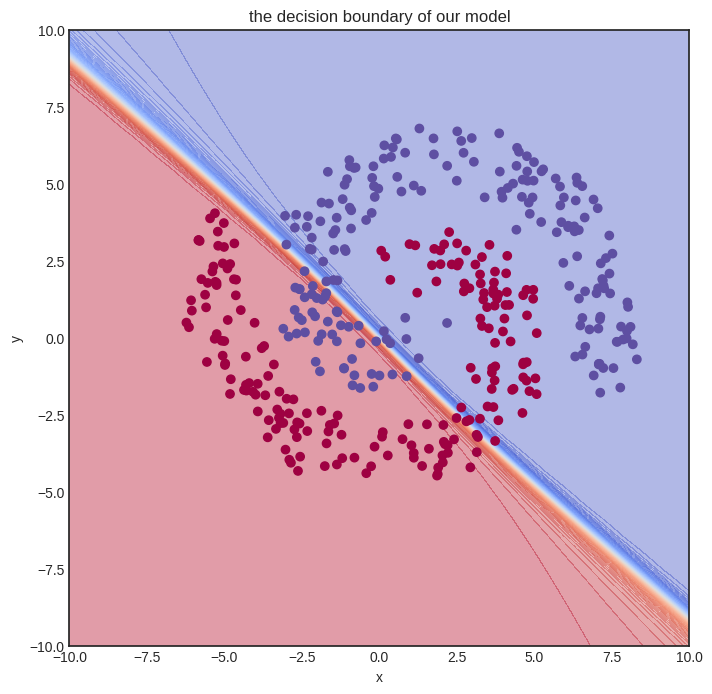
Training tensor networks is also much faster, as we shall see soon. Let’s initialize one and see how it looks.
model = TwoLayerNetwork()
from itertools import product


def visualize_model(model, xs, ys, res=100, xrange=(-10, 10), yrange=(-10, 10)):
    with plt.style.context("seaborn-v0_8-white"):
        plt.figure(figsize=(8, 8))

        res = 100
        x = np.linspace(xrange[0], xrange[1], res)
        y = np.linspace(yrange[0], yrange[1], res)
        xx, yy = np.meshgrid(x, y)
        zz = np.zeros_like(xx)

        for i, j in product(range(res), range(res)):
            zz[i, j] = model.forward(Tensor([xx[i, j], yy[i, j]])).value


        # plot the decision boundary
        plt.contourf(xx, yy, zz, levels=100, cmap='coolwarm_r', alpha=0.4)
        plt.xlabel('x')
        plt.ylabel('y')
        plt.title('the decision boundary of our model')

        # plot the data
        plt.scatter([x[0] for x in xs], [x[1] for x in xs], c=ys, cmap=plt.cm.Spectral, zorder=10)
        plt.show()

visualize_model(model, xs, ys)
/tmp/ipykernel_66116/4170422174.py:15: DeprecationWarning: Conversion of an array with ndim > 0 to a scalar is deprecated, and will error in future. Ensure you extract a single element from your array before performing this operation. (Deprecated NumPy 1.25.)
  zz[i, j] = model.forward(Tensor([xx[i, j], yy[i, j]])).value
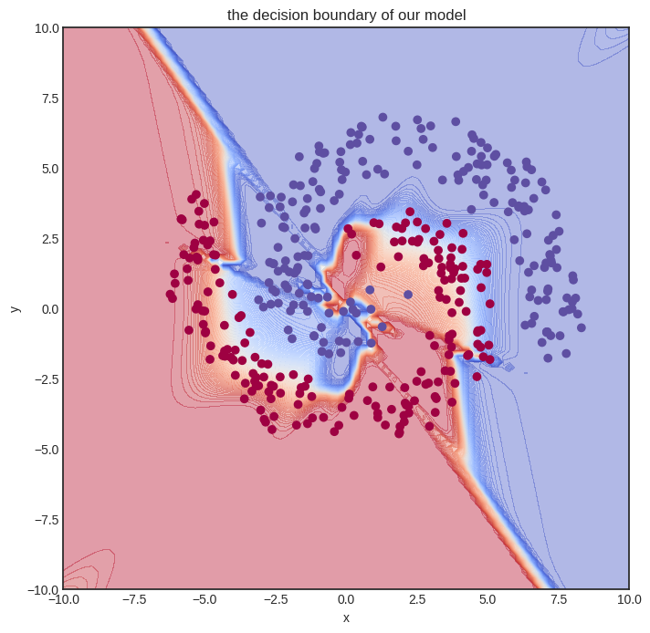
Here goes the training. We’ll let it rip and crunch out a whooping one hundred thousand iterations. For comparison, we merely did a thousand steps for the Scalar version, and even that almost made my notebook explode.
from mlfz.nn.tensor.loss import binary_cross_entropy


n_steps = 100000
lr = 0.1

for i in range(1, n_steps + 1):
    preds = model(xs)
    l = binary_cross_entropy(preds, ys)
    l.backward()
    model.gradient_update(lr)

    if i == 1 or i % 10000 == 0:
        print(f"step no. {i}, loss = {l.value}")
step no. 1, loss = 1.3500574656982025
step no. 10000, loss = 0.3276131190652927
step no. 20000, loss = 0.27962397222881064
step no. 30000, loss = 0.26929577387216247
step no. 40000, loss = 0.2990275403169361
step no. 50000, loss = 0.26435643969354067
step no. 60000, loss = 0.28143142115711317
step no. 70000, loss = 0.26137091793547507
step no. 80000, loss = 0.24449209263802452
step no. 90000, loss = 0.2385367334321998
step no. 100000, loss = 0.2446387078525447
In other words, despite having a more complex model and performing way more gradient descent steps, we are still much faster. Let’s time it to confirm. We’ll only measure a thousand training loops.
def train_model():
    model = TwoLayerNetwork()
    n_steps = 1000
    lr = 0.1

    for i in range(1, n_steps + 1):
        preds = model(xs)
        l = binary_cross_entropy(preds, ys)
        l.backward()
        model.gradient_update(lr)


%timeit -r 1 -n 1 train_model()
1.92 s ± 0 ns per loop (mean ± std. dev. of 1 run, 1 loop each)
And this is the final result.
visualize_model(model, xs, ys)
/tmp/ipykernel_66116/4170422174.py:15: DeprecationWarning: Conversion of an array with ndim > 0 to a scalar is deprecated, and will error in future. Ensure you extract a single element from your array before performing this operation. (Deprecated NumPy 1.25.)
  zz[i, j] = model.forward(Tensor([xx[i, j], yy[i, j]])).value
13.5. Tensor vs Scalar performance comparison#
Before moving on to the implementation details, let’s quickly compare the performance of Scalar vs. Tensor. To do that, we’ll use a simple one-layer neural network with thirty-two hidden neurons.
We’ll store the number of hidden neurons inside a variable so you can play around with it if you execute this notebook locally.
n_hidden_neurons = 32
First, here’s the data. Feel free to skip the code, it’s nothing we haven’t seen before.
import numpy as np
from mlfz.nn.scalar import Scalar
from mlfz.nn.tensor import Tensor

n_samples = 1000

xs_scalar = [[Scalar.from_random(), Scalar.from_random()] for _ in range(n_samples)]
ys_scalar = [Scalar.from_random() for _ in range(n_samples)]

xs_tensor = Tensor(np.array([[x1.value, x2.value] for x1, x2 in xs_scalar]))
ys_tensor = Tensor(np.array([y.value for y in ys_scalar]).reshape(-1, 1))
Our Scalar network takes quite a while to set up. Here we go:
from mlfz import Model
from mlfz.nn.scalar import functional as f_scalar
from itertools import product


class ScalarNetwork(Model):
    def __init__(self):
        self.A = [[Scalar.from_random() for j in range(n_hidden_neurons)]
                  for i in range (2)]
        self.B = [Scalar.from_random() for i in range(n_hidden_neurons)]

    def forward(self, x):
        fs = [sum([self.A[i][j] * x[i] for i in range(2)]) for j in range(n_hidden_neurons)]
        fs_relu = [f_scalar.tanh(f) for f in fs]
        gs = sum([self.B[i] * fs_relu[i] for i in range(n_hidden_neurons)])
        return f_scalar.sigmoid(gs)

    def parameters(self):
        A_dict = {f"a{i}{j}": self.A[i][j] for i, j in product(range(2), range(n_hidden_neurons))}
        B_dict = {f"b{i}": self.B[i] for i in range(n_hidden_neurons)}
        return {**A_dict, **B_dict}
To accurately measure the time of a single gradient step, we encapsulate all the logic into a single function called scalar_network_step.
from mlfz.nn.scalar.loss import binary_cross_entropy as bce_scalar


scalar_net = ScalarNetwork()


def scalar_network_step():
    preds = [scalar_net(x) for x in xs_scalar]
    l = bce_scalar(preds, ys_scalar)
    l.backward()
    scalar_net.gradient_update(0.01)
Let’s go and %timeit!
%timeit scalar_network_step()
372 ms ± 22.2 ms per loop (mean ± std. dev. of 7 runs, 1 loop each)
Now, about the Tensor network.
from mlfz.nn.tensor import functional as f_tensor


class TensorNetwork(Model):
    def __init__(self):
        self.A = Tensor.from_random(2, n_hidden_neurons)
        self.B = Tensor.from_random(n_hidden_neurons, 1)

    def forward(self, x):
        return f_tensor.sigmoid(f_tensor.tanh(x @ self.A) @ self.B)

    def parameters(self):
        return {"A": self.A, "B": self.B}
Look at that simplicity! Vectorization is worth it for that alone, but wait until we see how fast it is.
from mlfz.nn.tensor.loss import binary_cross_entropy as bce_tensor


tensor_net = TensorNetwork()


def tensor_network_step():
    preds = tensor_net(xs_tensor)
    l = bce_tensor(preds, ys_tensor)
    l.backward()
    tensor_net.gradient_update(0.01)
%timeit tensor_network_step()
4.71 ms ± 513 μs per loop (mean ± std. dev. of 7 runs, 100 loops each)
The actual performance depends on the machine this book is built on, but you should see a roughly 100x speedup, given by the magic of vectorization. If you are running this notebook locally, try changing the n_hidden_neurons variable in the first executable cell in this notebook. You’ll be surprised: the execution time of the Scalar version will rapidly increase, but the Tensor version will roughly stay the same!
That’s because the graph structure adds a heavy overhead to our computations. We’ll profile the code in a later version of the notebook, but this is because the actual computations like addition, multiplication, etc, are only a small portion of the training!